Building regulations 2025 - new non-domestic buildings: energy standard improvements - modelling report

2. Objective 1: Baseline models

Objective 1 is to establish the baseline from which to evaluate change. To achieve this, it is first necessary to establish the national build profile for Scotland for the analysis. This requires the derivation of a suitable number of representative building types and sub-types. Building types refer to the function of the building (office, school etc.) whilst sub-types represent distinct combinations of building type, heating fuel and Heating, Ventilation and Cooling (HVAC) strategy. The selected sub-types should be representative of the buildings added to the Scottish building stock over the last few years.

2.1 National Annual Building Profile for new Non-domestic Buildings

To derive the building sub-types an analysis has been undertaken of the EPC database, provided by the Scottish Government Building Standards Energy Policy Team, for new non-domestic building over the period from January 2021 to September 2024. This analysis and the resulting sub-types are described below.

The EPC database contains information on each of the circa 1,200 EPCs lodged during this period. This includes several parameters such as building type, floor area, EPC rating and some information about the building fabric and services.

The client requested that for the purposes of this project, the building types/models should be selected from those used to support changes to building regulations for England and Wales as shown below. These models are readily available, and it allows a comparison between national improvements.

Table 1: Building type models available from England and Wales.

England

• Office – deep plan, air conditioned
• Office – shallow plan, naturally ventilated
• Hotel
• Hospital
• Secondary School (includes sports facilities)
• Retail Warehouse
• Distribution Warehouse

Wales

• Office, air conditioned
• Office; naturally ventilated
• Hotel
• Integrated Health Care Centre
• Primary School
• A1 Retail (small food)
• Small Warehouse/ Industrial
• Medium Warehouse/ Industrial
• Large Warehouse/ Industrial
• Multi-Residential

The EPC database does not map directly to these building types but rather uses the building types embedded within SBEM which are based on the UK planning classification system. It was therefore necessary to map these planning classification categories to the building model types available; this mapping is shown in Table 2 and is based on building uses/profiles. In a small number of cases the mapping is a compromise (e.g. universities/colleges have been mapped to secondary school). In some cases, no logical mapping has been possible, however these cases account for less than 2% of the total floor area.

Table 2: Mapping of EPC database building types to model types, showing total database floor area.

EPC Database Building Types	Floor area (m²)	Floor area (%)	Model Types
Community/Day Centre	15,462	0.8%	NA
Education	241,590	12.9%	Secondary School
Emergency service	1,074	0.1%	NA
General Assembly/Leisure	59,682	3.2%	Retail
General Industrial	98,564	5.3%	Warehouse Distribution
Hospitals/Care Home	87,405	4.7%	Hospital
Hotel	179,249	9.6%	Hotel
Library/Museum/Gallery	7,391	0.4%	NA
Office/Workshops
Office/Workshop; Air Conditioning; Deep	414,402	22.1%	Deep Office AC
Office/Workshop; Mixed-mode with Natural Ventilation; Shallow	1,989	0.1%	Shallow Office NV
Office/Workshop; Heating and Natural Ventilation; Shallow	34,258	1.8%	Shallow Office NV
Office/Workshop; Air Conditioning; Shallow	8,630	0.5%	Shallow Office AC
Office/Workshop; Heating and Mechanical Ventilation; Shallow	7,278	0.4%	Shallow Office AC
Office/Workshop; Heating and Natural Ventilation; Deep	27,904	1.5%	Deep Office AC
Office/Workshop; Unconditioned; Shallow	1,457	0.1%	Shallow Office NV
Office/Workshop; Heating and Mechanical Ventilation; Deep	636	0.0%	Deep Office AC
Office/Workshop; Mixed-mode with Natural Ventilation; Deep	589	0.0%	Deep Office AC
Office/Workshop; Mixed-mode with Mechanical Ventilation; Deep	2,266	0.1%	Deep Office AC
Passenger terminal	6,968	0.4%	NA
Primary Healthcare Building	13,796	0.7%	Hospital
Residential school	30,855	1.6%	Hotel
Residential space	9,807	0.5%	Hotel
Restaurant/Cafes/takeaway	22,632	1.2%	Retail
Retail/Financial	187,088	10.0%	Retail
Secure Residential Institution	14,583	0.8%	Hospital
Standalone utility block	359	0.0%	NA
Storage/Distribution	204,322	10.9%	Warehouse Distribution
Universities/college	192,510	10.3%	Secondary School

Table 2 shows how the office building type has been split into sub-types which reflect the two building forms available in the English and Welsh models (deep-plan and shallow-plan). The EPC database does not directly make this deep/shallow-plan distinction, so a definition of deep and shallow plan has been based on the ratio of building floor area to building surface area which is available in the database.

On this basis it was found that the EPC database contains 145 sub-type combinations of mapped building type, heating fuel and HVAC strategy. However, for this analysis, it is sufficient to focus on the most common sub-types as these will allow sufficient determination of the impact of any changes to Building Standards – additional sensitivity analyses can be undertaken, if necessary, on less common, but important, sub-types.

Selection of the most prevalent sub-types was undertaken through focussing on the most dominant heating fuels and HVAC strategies. For this purpose, it was necessary to achieve at least 5% of the total floor area represented in the EPC database. Where less than 5% was achieved, the most similar dominant strategy was identified for the analysis (an alternative would be to pro-rata across all heating fuels/HVAC strategies).

The New Build Heat Standard (NBHS) prevents the use of direct emission heating in new buildings; however, came into force on 1 April 2024 which is during the period which EPC data has been analysed. Therefore, gas is still found to be the second most common heat source within new buildings. Gas-fired heating was removed from the build mix analysed during the later stages of this period, with the demand re-allocated on a pro-rata basis to air source heat pumps, direct electric, and district heating systems - to represent the likely transition away from direct emission to zero direct emission heating systems.

This mapping is shown in Table 3 and Table 4.

Table 3: Mapping of dominant heating fuel types.

Heat Source	Floor area (%)	Mapped Heating Fuel
Air Source Heat Pump	45.0%	Grid Supplied Electricity
Natural Gas	32.6%	Grid Supplied Electricity / District Heating
District Heating	5.5%	District Heating
LPG	1.2%	Grid Supplied Electricity / District Heating
Direct Electric	12.6%	Grid Supplied Electricity
Biomass	1.7%	Biomass
Oil	0.2%	Grid Supplied Electricity / District Heating
Ground Source Heat Pump	1.2%	Grid Supplied Electricity
Waste Heat	0.0%	Grid Supplied Electricity / District Heating

Table 4: Mapping of dominant HVAC strategies.

HVAC Strategy	Floor area (%)	Mapped HVAC Strategy
Air Conditioning	49.1%	Air Conditioning
Heating and Natural Ventilation	28.1%	Heating and Natural Ventilation
Heating and Mechanical Ventilation	20.9%	Heating and Mechanical Ventilation
Mixed-mode with Mechanical Ventilation	0.6%	Heating and Mechanical Ventilation

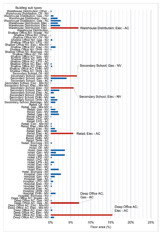
On this basis the number of building sub-types is reduced to 88, these are shown in Figure 1. This shows that only six building sub-types account for more than 5% of the total EPC database floor area; these are highlighted in yellow in Figure 1. A final round of selective mapping was then undertaken to group the remaining sub-types together into groups accounting for more than 5% of the total floor area. This process mapped non-dominant sub-types together into groups accounting for more than 5% of floor area or, in some cases, mapped these to sub-types that already accounted for more than 5% individually. This process results in the twelve sub-types shown in Table 5 these include seven building types, three heating fuels and three HVAC strategies. These twelve sub-types are assumed to comprise the national build mix for this analysis. Table 6 shows the extrapolated annual average build mix used to calculate the national carbon impacts presented in Section 4.4. Table 6 provides a summary of the key dimensions of the seven building types used in this analysis.

Table 5: Eleven building sub-types selected for analysis January 2021 to September 2024.

Building Sub-types	Floor Area (m²)	Floor Area (%)
Shallow Office; DHN; NV	104,306	5.7%
Deep Office AC; Elec; AC - HP	341,491	18.5%
Heath centre; DHN; MV	115,784	6.3%
Hotel; Elec; NV - DE	225,397	12.2%
Retail; Elec; AC - HP	113,208	6.1%
Retail; Elec; MV - HP	150,708	8.2%
Secondary School; DHN; AC	104,171	5.7%
Secondary School; Elec; MV - HP	233,658	12.7%
Secondary School; Elec; NV - DE	96,271	5.2%
Warehouse Distribution; Elec; AC - HP	101,873	5.5%
Warehouse Distribution; Elec; MV - DE	196,952	10.7%
Total	1,783,819	96.8%

Table 6: Eleven building sub-types selected for analysis annual average.

Building Sub-types	Floor Area (m²)	Floor Area (%)
Shallow Office; DHN; NV	107,754	5.85%
Deep Office AC; Elec; AC - HP	352,780	19.14%
Heath centre; DHN; MV	119,612	6.49%
Hotel; Elec; NV - DE	232,848	12.64%
Retail; Elec; AC - HP	116,950	6.35%
Retail; Elec; MV - HP	155,690	8.45%
Secondary School; DHN; AC	107,615	5.84%
Secondary School; Elec; MV - HP	241,382	13.10%
Secondary School; Elec; NV - DE	99,454	5.40%
Warehouse Distribution; Elec; AC - HP	105,241	5.71%
Warehouse Distribution; Elec; MV - DE	203,463	11.04%
Total	1,842,788	100.00%

Table 7: Sample building type summary of key dimensions.

Building Type	Floor area (m²)	Number of Storeys	External Wall Area (m²)	External Glazed Area (m²)
Deep-plan Office	12,100	5	4,000	1,500
Health centre	2,089	2	1,352	138
Hotel	1,087	3	903	319
Secondary School	8,012	3	4,416	1,271
Retail	1,250	1	600	60
Shallow-plan Office	2,160	3	1,218	487
Distribution Warehouse	5,262	Warehouse=1 storey Integral office=2 stories	2,463	684

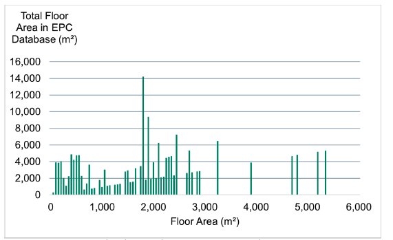
In general, the building models will be those used for similar building regulations analysis in England. The one exception is the retail category where there was further investigation as to whether it is best represented by the small retail unit used for analysis in Wales or the larger retail warehouse used for the English analysis. The Welsh retail unit is a small, detached retail building with a small office and storage and has a floor area of 1,250m² and the English retail warehouse is a detached building including a large retail floor and back-of-house office and other staff facilities including changing rooms and kitchen with a total floor area of 5,262m². Figure 2 shows the floor area distribution of the retail building category in the EPC database. This shows that there is a small number of retail units with large floor areas (seven buildings have a floor area greater than 3,000m²) but most retail floor area is in units with floor areas between 1,000m² and 3,000m². On this basis it is recommended that the smaller Welsh retail unit model is used for this analysis as its floor area falls within this range.

2.2 Baseline specification

To derive a baseline 2023 compliant specification for the sample buildings identified in the national profile above, as a default the specifications are based on the Section 6 2023 notional building values for the relevant fuel type. These values have been modified to reflect common practice where it is found to differ from the Section 6 2023 notional building values/approach.

The modifications have been informed by a review of EPC data made available by Scottish Government. There is significant variation in the design specifications used in projects, hence many projects do not simply adopt the values in the notional building. To identify tendencies for a significant difference between actual buildings and the values used in the notional building, a data analysis has been undertaken to identify potential differences. The notional building values have been changed if they are in the lower quartile of energy performance (0 to 25%) or upper quartile of energy performance (75 to 100%) of the EPC database distribution i.e. do not tend to be common practice. In such cases, a value around the median has been adopted.

Any amendments proposed to the baseline specifications from that given in the notional 2022 building(s) have been agreed with Scottish Government, and modelled BDERs are kept within 1% of the TDER, see Section 2.3.

The non-domestic EPC database does not contain the same level of detailed information as is present in the domestic EPC database and so fewer conclusions can be drawn from it.

Several anomalies were identified in the database, and these cases have been excluded from the analysis described below to derive a robust sample of EPCs from which conclusions can be drawn. The following steps were taken to remove anomalies prior to analysis:

• All EPCs lodged prior to the January 2021 were removed. The current version of Section 6 came into effect from 1 February 2023, with the NBHS coming into force in 1 April 2024. To provide a suitably large dataset, the earliest date for EPCs included within this analysis has been extended to cover some buildings designed and constructed to meet an earlier version of Section 6. Furthermore, given the transitional arrangements and the length of typical design and construction programmes EPCs lodged for several months after the current version came into force (1 February 2023, with NBHS updates in 1 April 2024) are likely to have been compliant with earlier versions of the regulation.
• EPC records which appear to fail to comply with Section 6 (i.e. TER
• Several EPC records were identified which showed the notional building average U-value to be zero. The reason for this is not apparent, however these cases have been removed from the analysis.
• Unconditioned buildings have been removed from the analysis.

Naturally ventilated buildings have been analysed separately from mechanically ventilated/ cooled buildings to assess the effect of the differences in energy demand balances.

For each regulated end use (heating, cooling, ventilation, lighting and domestic hot water) along with renewable energy generation, a summary of the relative performance of the actual and notional buildings is provided. This is done by comparing the actual energy consumption divided by the notional energy consumption, so that a ratio of less than 100% means that the actual building has a lower energy demand than the notional building and vice-versa for ratios greater than 100%. For some end uses, including lighting, ventilation and domestic hot water, the EPC database does not contain detailed data so analysis is limited to this ratio.

2.2.1 Building Fabric: Air tightness, U-values and Thermal Bridging

The EPC database does not contain information on individual building elements (walls, windows etc.), rather the database contains the following metrics:

• Air tightness;
• Average (area-weighted) building U-value for the whole building envelope;
• Average building thermal bridging (alpha-value).

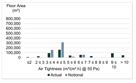
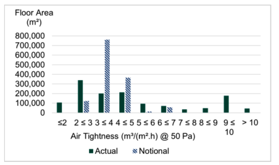
Figure 3 and Figure 4 show the distribution of air tightness values for naturally ventilated and mechanically ventilated/cooled buildings, compared to the notional building.

The distributions are similar; however, mechanically ventilated buildings are seen to more commonly have lower (better) levels of air tightness, with the most common result being 2 to 3 m³/m².hr at 50Pa. The distribution for mechanically ventilated buildings shows a longer tail towards the poorer levels of air tightness. By comparison, naturally ventilated buildings are seen to most commonly have air tightness results between 4 and 5 m³/m².hr at 50Pa, with a shorter tail towards the poorer air tightness results.

Under Section 6 (2015), the infiltration rate applied to the notional building depended on the building type and area, and servicing type, and varied from 3 to 7 m³/m².hr at 50Pa. Under the current Section 6 (2022) all notional building use an infiltration rate of 4m³/m².hr at 50Pa.

The EPC database includes six records where the notional building has an infiltration rate of 0m³/m².hr at 50Pa, which is likely to be an error either in the record or modelling. There are 875 records where the notional building’s infiltration rate is between 3 and 7m³/m².hr at 50Pa (but not exactly 4m³/m².hr at 50Pa), and although the most recent record was lodged on 19/09/2024, it is hypothesized that these records relate to buildings assessed against Section 6 (2015). There are 293 records where the notional building’s air permeability is exactly 4m³/m².hr at 50Pa, with certification dates between 08/02/2023 and 30/09/2024, indicating that these buildings have been assessed against the current Section 6 (2022).

On this basis the air tightness for the compliant solutions is set to 5m³/m²/hr @ 50Pa.

The building average U-value gives only a limited insight into the individual U-values being used for the different fabric elements. Buildings with large amounts of glazing will tend to have higher average U-values than those with less glazing even if the U-values of individual elements are similar. Similarly, those with different built forms will have a different average U-value if a certain envelope element (e.g. wall) takes up a greater or less proportion of the total surface area.

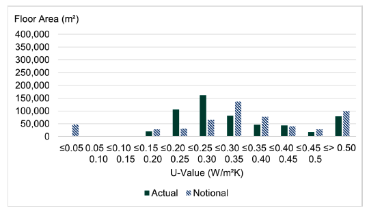
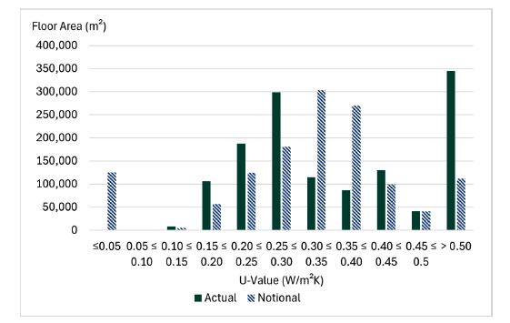
Some overall insight is provided by comparing the average U-value of the actual and notional buildings. Figure 5 and Figure 6 compare the actual and notional average U-values for naturally ventilated and mechanically ventilated/cooled buildings respectively. Both graphs show that there is a tendency for the U-values of the actual buildings to be lower (i.e. better) than those of the notional buildings, however this tendency appears to be slight.

The below graphs show a proportion of notional buildings where the average U-value is less than 0.05W/m²K, indicative of a very highly performing building fabric. Upon further investigation of the EPC database, this relates to 40 buildings which are recorded with a building average U-value of 0.000 W/m²K. There does not appear to be a reasonable cause for this, for example buildings without external surfaces such as a unit in a larger development, as the affected records are for buildings of a range of sizes (79 to 19,362m²) and functions. Therefore, it is hypothesized that the recorded 0.000 W/m²K is an error, either in the modelling or recording.

On this basis the U-values for the compliant solutions are set to replicate the current notional building specification.

The EPC database contains records for EPCs generated through both SBEM and Dynamic Simulation Modelling (DSM) software. SBEM requires that the user inputs thermal bridging values on an individual basis (or uses default values). However, in DSM software, non-repeating thermal bridges are generally input as a simple percentage adjustment to U-values, the default value for the actual building is 25% under Section 6 (2023), compared to 10% under Section 6 (2015). In both regulations, the adjustment applied in the notional building is 10%.

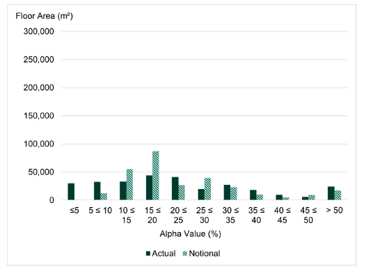
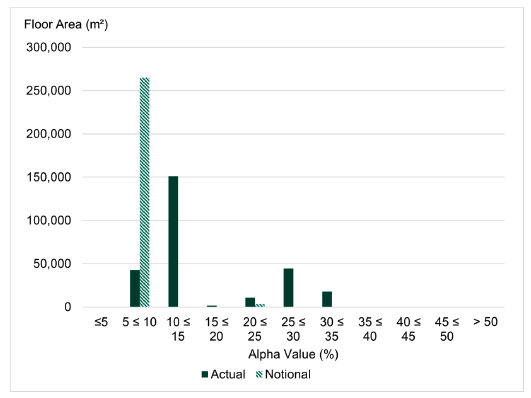
Figure 7 and Figure 8 compare the actual and notional thermal bridging values for naturally ventilated buildings as recorded in SBEM and DSM generated EPCs, respectively. Figure 9 and Figure 10 show the same data for mechanically ventilated buildings.

No clear trend is evident in these graphs. However, it appears that thermal bridging in actual buildings tends to be a little better than notional buildings. The median values for the actual and notional buildings with natural ventilation are 23.8% and 22.3% respectively. For buildings with mechanical ventilation/cooling, these values are 22.4% and 19.9% respectively. This suggests that there is not much variation in thermal bridging in relation to the building servicing strategy.

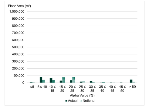
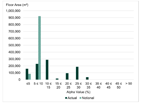
As the difference between the actual and notional buildings appears relatively small, the thermal bridging for the compliant solutions are set to replicate the current notional building specification.

2.2.2 Building Services: HVAC strategy

The EPC database contains some limited information on individual building service efficiencies. Heating and cooling efficiencies are included in the database; however no other building service parameters can be viewed directly. The EPC database does include data on the modelled energy demand of each end use (heating, cooling, hot water, lighting and fans and pumps), and some conclusions may be drawn from this data.

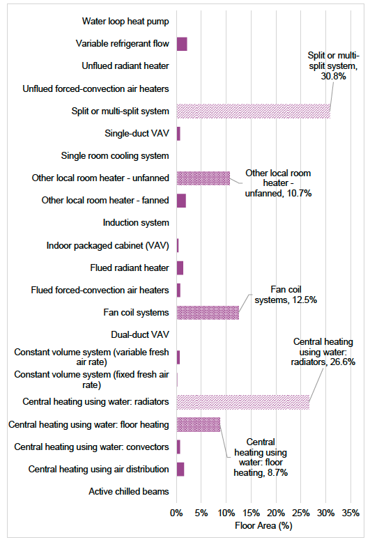
The range of realistic efficiencies for building services is strongly influenced by the type of system installed. Analysis of the different HVAC system types recorded in the EPC database is shown in Figure 11. This shows that two system types dominate (hatched with diagonal lines in Figure 11):

• Split or multi-split heating and cooling (30.8% of floor area).
• Central heating using radiators (26.6% of floor area).

There are a further three popular system types that are used within a similar proportion of buildings (shown in light green in Figure 11):

• Fan coil heating and cooling (12.5% of floor area).
• Unfanned local room heaters (10.7% of floor area).
• Underfloor heating (8.7% of floor area).

The remaining system types are each used in 2.1% or less of the floor area.

2.2.3 Building Services: Heating generators

The efficiency of a heating system is strongly influenced by the type of heat generator in use. For example, the typical efficiency of a gas boiler is between 85% and 95%, whereas for a heat pump the typical efficiency is much higher (usually between 3 and 6, i.e. 300% to 600%).

Figure 12 shows the percentage floor area in the EPC database which is heated by each heat generator type from all EPCs lodged between January 2021 and September 2024, with Figure 13 showing the data from the subset of EPCs lodged between 1 April 2024 and September 2024, after the New Build Heat Standard (NBHS) came into force.

Buildings served by LTHW boilers in the EPC database are recorded as being fuelled by natural gas, LPG, biomass, oil and waste heat.

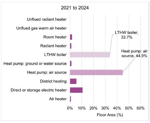
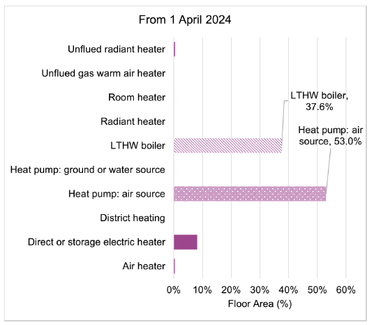
The implementation of the NBHS has not yet led to a marked transition away from LTHW boilers, which are predominantly natural gas-fired, towards other clean heat sources.

The proportion of buildings served by different heat sources are similar for the 2021 to 2024 period as to that since 1 April 2024 when the NBHS has been in force. This is potentially due to the long timelines associated with the design and construction of buildings which means that most, if not all, of the buildings with EPCs lodged between 1 April 2024 and October 2024 would not have been impacted by the implementation of the New Build Heat Standard.

As previously discussed, to align with the NBHS and to reflect the new-build mix, the baseline buildings will use one or more of the following heat sources:

• Electric air source heat pump,
• District heating, or
• Direct electric heating.

2.2.4 Building Services: Air Source Heat Pumps (for heating)

The efficiency of air source heat pumps is strongly influenced by whether they deliver heat as hot water or warm air. The data recorded in the EPC database does not explicitly differentiate between ASHP systems drawing heat from outside air to serve water-based systems and those that can move heat within buildings and use refrigerant as the working fluid (Variable Refrigerant Flow – VRF or split systems). However, this differentiation can be inferred from the NCM system type. The relative efficiency of air-to-water and air-to-air heat pumps have been analysed by assigning the NCM system types as shown below.

Heat pump type: Air to Water

• Central heating using air distribution
• Central heating using water: convectors
• Central heating using water: floor heating
• Central heating using water: radiators
• Constant volume system (variable fresh air rate)
• Fan coil systems
• Indoor packaged cabinet (VAV)
• Induction system
• Single-duct VAV

Heat pump type: Air to Air

• Dual-duct VAV
• Flued radiant heater
• Other local room heater – unfanned
• Single room cooling system
• Split or multi-split system
• Variable refrigerant flow
• Water loop heat pump

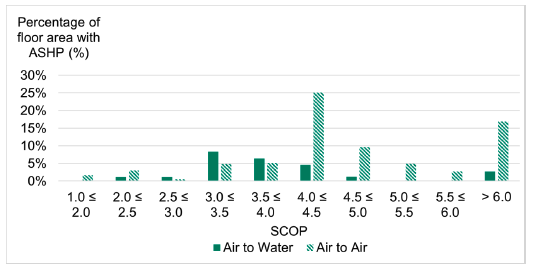
Figure 14 and Table 8 show the distribution of ASHP efficiencies for wet heating systems only (air-to-water heat pumps) and those delivering warm air (air-to-air heat pumps), by floor area, across all building types.

The current notional building seasonal heating efficiency for ASHPs is 300% (SCOP = 3). The data shows that this falls below the 25^th percentile in the EPC database for both air-to-water and air-to-air heat pumps and is therefore not deemed representative of current build specifications.

Whilst VRF and split systems are often more efficient, ASHPs serving wet systems are more widely suitable to the new non-domestic building stock than VRF and split systems. For example, VRF and split systems are generally deemed inappropriate for clinical applications due to difficulty in cleaning. They are also more limited by the maximum pipe length they can accommodate (although this is increasing as technology develops). Hence, if ASHPs are to be included in the new notional building, it appears sensible to specify the performance standard based on characteristics of those ASHPs serving wet systems.

Rather than adopting different SCOP values for air-to-water and air-to-air heat pumps, the baseline buildings use a SCOPO of 3.5, which is the median value for air to water heat pumps.

Table 8: ASHP heating SCOP percentiles.

Percentile	Air to Water	Air to Air	All ASHP
75th	4.0	4.6	4.5
50th	3.5	4.2	4.0
25th	3.2	3.5	3.3

The EPC database does not contain information on the heating system flow temperatures assumed, and for most heat sources this variable has a minor impact. However, ASHP efficiency is strongly influenced by the temperature which it is supplying; this matter is discussed in detail in Section 3.1.3.

The influence of flow temperature on ASHP operating efficiency is acknowledged in the current Part L 2021 requirements for England, which require that space heating systems are designed to operate at a maximum flow temperature of 55ºC. This both facilitates the efficient operation of heat pumps where used, and for fossil fuelled heating systems allows for future heat pump retrofit with less disturbance to the building and its systems. Section 6 does not currently contain a similar limit, with the NBHS requiring the use of heat pumps in most buildings; so that designers are incentivised to use flow temperatures that support their efficient operation.

Under the NBHS, bioenergy heating systems, such as wood burners and peat-burning systems, are still permitted. These systems would unlikely benefit from flow temperatures being reduced to 55ºC, although should be low enough to allow the system to operate in condensing mode.

2.2.5 Building Services: Heating

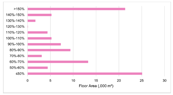
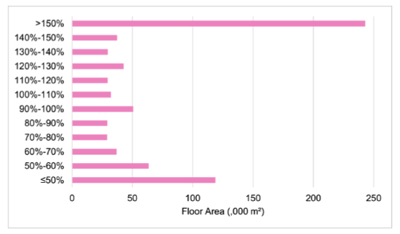
The overall performance of the space heating in the actual and notional buildings has been analysed as described previously.

This shows that for buildings that are:

• Naturally ventilated: Most commonly, the actual building’s energy consumption is either much lower (<50%) or much higher than the notional building (>150%).
• Mechanically ventilated/cooled: Most commonly, the actual building’s energy consumption is much greater than the notional building (<150%). The next most common situation is for the actual building’s energy consumption to be much lower than the notional building.

2.2.6 Building Services: Cooling

As for ASHPs delivering space heating, the EPC database does not differentiate between wet cooling systems (air-to-water), using chilled water, and those using refrigerant as the working fluid (air-to-air). As for heating, the NCM system type is used to infer the chiller type; with the NCM system allocation as shown in Section 2.2.4 noting that only systems that provide cooling are included in this analysis.

Within the EPC database, there are 435 buildings recorded with air conditioning (cooling) as the primary servicing type (total floor area of 915,958m²). However, of these buildings there are 64 buildings (floor area of 260,883m²) who’s cooling SEER is recorded as zero. It is unclear the reason for these entries, however, to allow meaningful analysis of the data, these have been screened out from subsequent analyses.

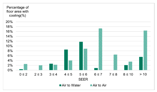
The notional SEER for cooling systems is 6.4. Figure 17 and Table 9 show that this falls between the 50^th percentile and 75^th percentile recorded in the EPC database for all cooling types and for air-to-air systems; however, the notional SEER exceeds the 75^th percentile for air-to-water systems.

There is a significant spread in cooling energy performance; most commonly the actual building’s cooling energy consumption is less than the notional building, however there are significant examples of the actual building’s cooling energy being much greater (poorer) than the notional. This suggests that other design features, for example glazed area, help to reduce the cooling energy consumption, despite the cooling SEER typically being poorer than the notional building’s SEER of 6.4.

Table 9: Cooling SEER percentiles.

Percentile	Air to Water	Air to Air	All cooling
75th	5.6	6.7	6.5
50th	5.5	5.8	5.6
25th	4.4	4.0	4.2

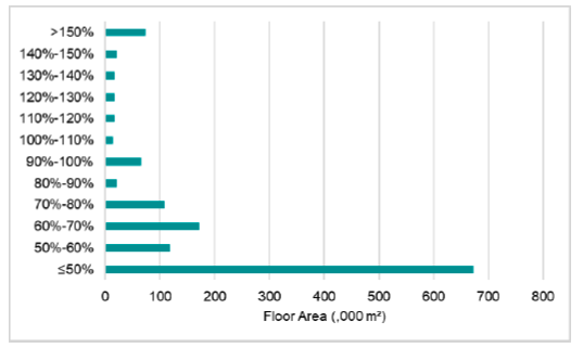
The overall performance of the cooling in the actual and notional buildings has been analysed as described previously.

This shows that for buildings that are:

• Mechanically ventilated/cooled: Most commonly the actual building’s energy consumption is less than the notional building. However, there is a significant proportion of buildings where the actual building’s cooling energy is much greater than the notional building.

2.2.7 Building Services: Fans and Pumps

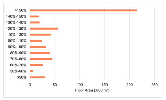
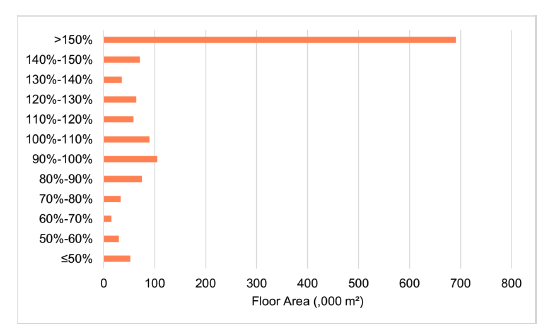
The overall performance of the auxiliary (fans and pumps) energy in the actual and notional buildings has been analysed as described previously. The EPC database does not record detailed performance metrics; therefore, the analysis is limited to considering the ratio of actual to notional building’s energy consumption.

This shows that for buildings that are:

• Naturally ventilated: Tendency for the actual building’s energy consumption to be significantly higher than the notional building.
• Mechanically ventilated/cooled: Tendency for the actual building’s energy consumption to be significantly higher than the notional building.

In naturally ventilated buildings, auxiliary energy use will predominantly relate to pumping energy. Therefore, the data suggests that the actual building typically uses a less energy efficient variable speed pumping control type than is adopted in the notional building. This factor may contribute to the relationship seen for mechanically ventilated and cooled buildings, but in this group the auxiliary energy will likely be dominated by ventilation fan energy. Therefore, for mechanically ventilated and cooled buildings, the data suggests that actual buildings may be using fans with poorer (higher) SFPs and/or ventilation systems with less demand control.

2.2.8 Building Services: Lighting

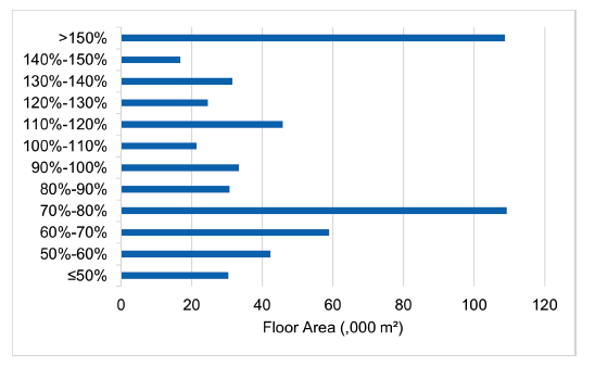
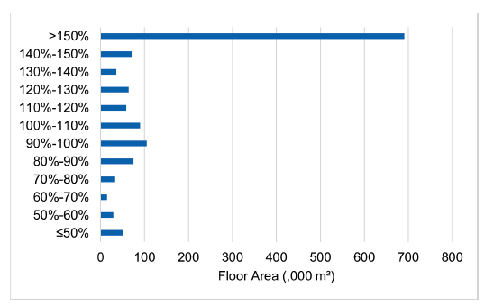
The overall performance of the lighting in the actual and notional buildings has been analysed as described previously. The EPC database does not record detailed performance metrics; therefore, the analysis is limited to considering the ratio of actual to notional building’s energy consumption.

This shows that for buildings that are:

• Naturally ventilated: The actual building’s lighting energy consumption is most commonly much higher than the notional building (>150%), or slightly better than the notional building (70% - 80%).
• Mechanically ventilated/cooled: Tendency for the actual building’s energy consumption to be significantly higher than the notional building.

Where the actual building’s lighting energy consumption is higher than the notional building (>100%), this may be due to the actual building design using luminaires with lower efficacies and/or less automatic control. Where the actual building’s lighting energy consumption is lower than the notional building’s (<100%), this is most likely due to higher efficacy fittings being used.

2.2.9 Building Services: Domestic Hot Water

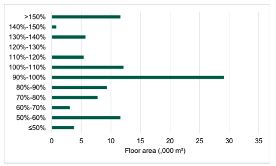
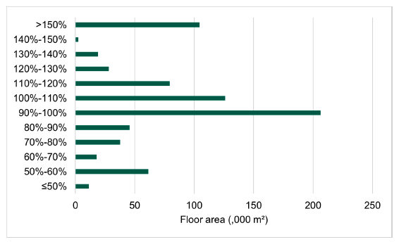
The overall performance of the domestic hot water in the actual and notional buildings has been analysed as described previously. The EPC database does not record detailed performance metrics; therefore, the analysis is limited to considering the ratio of actual to notional building’s energy consumption.

This shows that for buildings that are:

• Naturally ventilated: Tendency for the actual building’s domestic hot water energy consumption to be similar to the notional building (90% - 100%).
• Mechanically ventilated/cooled: Tendency for the actual building’s domestic hot water energy consumption to be similar to the notional building (90% - 100%).

Therefore, the data suggests that the efficiency of DHW systems in actual buildings, accounting for both the generator efficiency and the storage and circulation losses (if applicable), are similar to those in the notional building.

2.2.10 Renewable Energy Generation

Increasingly, renewable electricity generating technologies, typically photovoltaic panels, are included in buildings as part of the design solution to achieve compliance with the current version of Section 6.

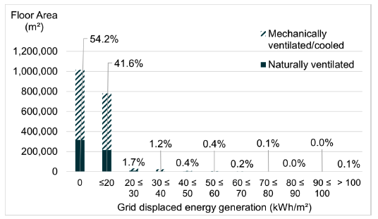
The EPC Database records the amount of electricity generated by PV, in kWh per m² of building floor area, with the distribution illustrated in Figure 25.

For both naturally and mechanically ventilated/cooled buildings, approximately 55% of buildings (by floor area) do not benefit from any PV electricity generation. Where buildings do have PV installed, it is most common for these to generate less than 20kWh/m² of building floor area. Approximately 0.17% of buildings, by floor area, benefit from PV that generates more than 60kWh/m² of building floor area.

Table 10 illustrates the percentile values for PV electricity generation per m² of building floor area.

Table 10: PV electricity generation.

Percentile	PV electricity generation (kWh/m² of floor area per year)
75th	26.6
50th	12.2
25th	6.0

The EPC database does not record the efficiency of the PV panels installed in the buildings; and it is not possible to infer the efficiency of the panels installed on buildings from their output. However, the range of market-available PV panels and inverters available are limited and tend towards similar efficiencies, for example panels circa. 20% efficient and inverters circa. 95% efficient. It is, therefore, more likely that a building’s architecture is the key driver behind differences in PV panel output, where a tall, narrow building (e.g. a high-rise tower) typically has a smaller proportional area available for PV installation compared to a low-rise building, where the roof area is proportionally greater. Table 16 outlines the PV areas included in the baseline buildings to achieve compliance.

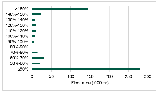
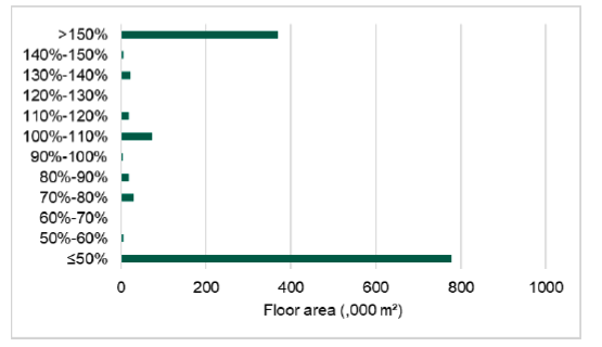
The overall contribution of zero carbon electricity generation in the actual and notional buildings has been analysed as described previously.

This shows that for buildings that are:

• Naturally ventilated: Most commonly the actual building generates much less energy than the notional building (<50%). The next most common situation is for the actual building to generate much more energy than the notional building (<150%).
• Mechanically ventilated/cooled: Most commonly the actual building generates much less energy than the notional building (<50%). The next most common situation is for the actual building to generate much more energy than the notional building (<150%).

2.3 Baseline Compliant Specifications

The following table outlines the baseline modelling specification, representing the current business as usual (BAU) approach to achieving Section 6 compliance as described in previous sections.

Table 11 – Table 15 show the business as usual (baseline) modelling specification, compared to the current Section 6 (2023) notional building specification. Values that deviate from the notional building specification are highlighted in yellow.

Where required, the area of PV has been modified to achieve a BDER within 1% of the TDER as shown in Table 16; noting that none of the modelled buildings include direct emissions heating systems and therefore are not required to comply with the carbon dioxide emissions target (TER).

Table 11 : Business as Usual (Baseline) Modelling Specification.

Variable	Section 6 2022 notional	Business as Usual
Wall U-Value (W/m²K)	0.15	0.15
Roof U-Value (W/m²K)	0.11	0.11
Floor U-Value (W/m²K)	0.13	0.13
Window U-Value (W/m²K)	1.20	1.20
Window G-value	0.50	0.50
Window Light Transmittance	0.77	0.77
Rooflight U-Value (W/m²K)	1.90	1.90
Rooflight G-value	0.50	0.50
Rooflight Light Transmittance	0.77	0.77
Thermal Bridging	As per NCM guide paragraphs 106, 107 and table 9	As per NCM guide paragraphs 106, 107 and table 9
Air Tightness (m³/m².hr at 50Pa)	4	5

Table 12: Business as Usual (Baseline) Modelling Specification - Heating & Cooling.

Variable	Section 6 2022 notional	Business as Usual
ASHP Heating SCOP Based on Air to Water (including 10% in-building delivery losses)	3.00	3.15 Flow Temp @ 55°C
Direct Electric SCOP	Natural gas – SCOP = 93% (including 10% in-building delivery losses)	100%
District Heating Heating SCOP	Natural gas – SCOP = 93% (including 10% in-building delivery losses)	90% Flow Temp @ 55°C (including 10% in-building delivery losses)
Cooling SEER	6.4 (SSEER = 5.1)	5.5 (SSEER = 4.4)

Table 13: Business as Usual (Baseline) Modelling Specification - Domestic Hot Water.

Variable	Section 6 2022 notional	Business as Usual
High Demand: Heat Pump	2.70	3.25
High Demand: Direct Electric	Natural gas – 93%	100%
High Demand: District Heating	Natural gas – 93%	100%
Low demand: Direct Electric	100%	100%

Table 14: Business as Usual (Baseline) Modelling Specification - Lighting & Ventilation.

Variable	Section 6 2022 notional	Business as Usual
Lighting Luminaire (lm/cW)	95	95
Daylight Lighting Control	All rooms that receive daylight directly (i.e. have an external window	All rooms that receive daylight directly (i.e. have an external window
Occupancy Lighting Control	Manual-On-Auto-Off	Manual-On-Auto-Off
Parasitic Power	0.1	0.1
Display Lighting (lm/cW)	95	95
Display Lighting Control	None	None
Central ventilation SFP (W/l/s)	1.80	1.80
Terminal unit SFP (W/l/s)	0.30	0.30
Ventilation Heat Recovery	76	76
Demand Control Ventilation	Demand control of ventilation through variable fan speed control based on CO2 sensors	Demand control of ventilation through variable fan speed control based on CO2 sensors
Variable speed pumping	Variable speed pumping with multiple pressure sensors in the system	Variable speed pumping with multiple pressure sensors in the system

Table 15: Business as Usual (Baseline) Modelling Specification - PV Area.

PV Area Lesser of	Section 6 2022 notional	Business as Usual
% of conditioned GIA	15%	Modified to achieve a BDER within 1% of the TDER 30% [1]
% of foundation area	30%	Modified to achieve a BDER within 1% of the TDER 30% [1]

Table 16: PV panel areas included in Baseline Models.

Building	PV Area (m²)	Percentage of Conditioned GIA	Percentage of Roof Area
Shallow Office AC; DHN; NV	282.90	13%	39%
Deep Office AC; Elec; AC - HP	594.52	5%	25%
Health centre; DHN; MV	476.33	24%	41%
Hotel; Elec; NV - DE	0	0%	0%
Retail; Elec; AC - HP	70.85	6%	6%
Retail; Elec; MV - HP	30.62	2%	2%
Secondary School; DHN; AC	1,593.94	20%	61%
Secondary School; Elec; MV – HP	389.25	5%	15%
Secondary School; Elec; NV - DE	2,165.98	27%	83%
Warehouse Distribution; Elec; AC – HP	1,782.30	34%	25%
Warehouse Distribution; Elec; MV - DE	2,402.33	46%	34%

2.3.1 Key results from Baseline Compliant Specifications

The following table outlines the key results from the baseline modelling, as calculated in SBEM v6.1.e. As all modelled buildings use zero direct emission heating sources, compliance is demonstrated by meeting the Target Delivered Energy Rate.

The BAU specification is based on evidence from the EPC database and so does not align with the current notional building. The breakdown of energy uses for individually buildings vary widely with building design and the functions and sizes of individual spaces. Therefore, the energy performance of the BAU specification does not always achieve compliance with the current Building Regulation for the eleven archetypes modelled for this analysis.

The naturally ventilated hotel using direct electric heating is found to comply with the Delivered Energy Rate without the inclusion of PV; therefore, its pass margin is 2.2%. All other buildings are found to require a contribution from PV to achieve compliance and in those cases, the area of PV has been calculated to achieve a 0% pass.

Table 17: Key Compliance Results from Baseline SBEM models.

Building	BDER (kWh/m²)	TDER (kWh/m²)	Delivered Energy Pass Margin (%)
Shallow Office; DHN; NV	18.21	18.21	0.0%
Deep Office AC; Elec; AC - HP	28.50	28.50	0.0%
Heath centre; DHN; MV	12.86	12.86	0.0%
Hotel; Elec; NV - DE	265.27	271.11	2.2%
Retail; Elec; AC - HP	63.56	63.56	0.0%
Retail; Elec; MV - HP	27.52	27.52	0.0%
Secondary School; DHN; AC	32.50	32.50	0.0%
Secondary School; Elec; MV - HP	26.55	26.55	0.0%
Secondary School; Elec; NV - DE	27.95	27.95	0.0%
Warehouse Distribution; Elec; AC - HP	43.39	43.39	0.0%
Warehouse Distribution; Elec; MV - DE	38.58	38.58	0.0%

For comparison purposes only, as carbon dioxide emissions are no longer used as a compliance metric for buildings using zero direct emissions heating systems, the resulting carbon dioxide emission rates have been calculated for the above scenarios, as reported in Appendix B.

Table 18: Breakdown of Actual Building Delivered Energy (kWh) for Baseline Buildings.

Building	Heating (kWh)	Cooling(kWh)	Aux. (kWh)	Light. (kWh)	DHW (kWh)	Useful PV output (kWh)
Shallow Office; DHN; NV	56,000	0	2,180	17,851	5,765	42,468
Deep Office AC; Elec; AC - HP	20,743	72,857	179,154	126,714	31,739	89,245
Heath centre; DHN; MV	49,387	16	14,596	22,416	6,779	67,529
Hotel; Elec; NV - DE	86,830	0	2,351	9,266	183,464	0
Retail; Elec; AC - HP	3,685	41,873	23,031	19,441	2,051	10,636
Retail; Elec; MV - HP	7,613	0	9,892	19,441	2,051	4,596
Secondary School; DHN; AC	108,896	23,896	135,218	61,301	153,808	222,689
Secondary School; Elec; MV - HP	57,664	620	60,315	61,301	91,288	58,432
Secondary School; Elec; NV - DE	232,216	565	90,280	61,301	131,336	291,753
Warehouse Distribution; Elec; AC - HP	63,144	24,617	345,908	23,185	38,995	267,548
Warehouse Distribution; Elec; MV - DE	347,910	0	41,242	23,185	79,214	288,542

2.4 Passivhaus Planning Package Modelling Comparison

2.4.1 Context

The Scottish Government aims to understand how the business-as-usual performance might differ across different compliance engines. SBEM v7 is the proposed compliance calculations methodology for determining compliance against Section 6 of the Non-domestic technical handbook for Scotland. However, the Scottish Government has been challenged by industry to explore routes for allowing alternative methods of calculation, namely Passivhaus Planning Package (PHPP). The way in which PHPP could be applied for building regulations compliance calculations needs to be understood.

In addition to differences in the building physics algorithms, PHPP requires significantly more detailed data inputs than are required for SBEM calculations. Therefore, a decision would be needed on the level of data entry that is required for an alternative compliance calculation. A differing level of input data may result in the regulations of building elements and systems designs which are not currently directly regulated by SBEM. For example, HVAC ducting design is an input for PHPP, whereas ventilation duct losses are simply a factor in SBEM.

PHPP also applies a different environmental standardisation compared to SBEM, this predominantly takes the form of weather data, internal heat gains and heating and cooling schedules. Therefore, the BAU performance in PHPP will be significantly impacted by the standardisation as well as the level of data entry.

To enable a meaningful comparison of results between PHPP and SBEM, the PHPP modelling approach has been to align with the SBEM assumptions as far as possible. It is noted that this does not represent a certifiable PHPP model result. Therefore, the impacts of PHPP data requirements, conventions of data collection/measurement and standardisation will be discussed qualitatively.

2.4.2 Approach

To establish a set of BAU archetypes, Passivhaus Planning Package version 10.6 was used to model these buildings. The following modelling approaches have been used to create a like for like model comparison. Such a comparison will help to identify how the underlying building physics algorithms in PHPP and SBEM differ.

Weather data

SBEM weather data is based on the CIBSE published TRY 2016 files for specific regions. The SBEM modelling presented in this report utilised the Glasgow TRY. PHPP uses its own weather data, which is specifically formatted to support the PHPP building physics calculations. The closest weather station data to Glasgow in PHPP is the Glasgow airport data; therefore, this was used for the PHPP modelling.

Model Geometry

The geometry for each archetype has been aligned with the inputs of the SBEM models, this is therefore based on internal dimensions rather than the external dimensions that PHPP conventions require. Given the scale of the buildings modelled, the additional heat loss associated with this difference in conventions is small and not expected to significantly change the results.

Thermal performance of building elements

The thermal performance of each building unique opaque element has been input into the PHPP as a single average value, (i.e. a U-value that represents the full build up including the internal and external heat transfer coefficients). For certification purposes, PHPP requires opaque elements such as walls, roofs and floors to be input as a full build up within the in-situ one-dimensional heat loss calculations. It is important to note that PHPP does not require the individual element thermal mass to be input, rather, it uses a whole building thermal mass parameter, which is set based on a high-level description of the building structure. Therefore, no impact on thermal mass calculations is expected by only inputting a single element U-value in place of the full build up.

For glazed elements, the U-value for the whole window has been applied to the glazing and the frame. Frame factors have been aligned between SBEM and PHPP, to achieve this a standard window size of 1m² has been used in PHPP and the frame width set to achieve the SBEM frame factor ratio. The number of 1m² windows per orientation has been set in PHPP to equal the total amount of window area per orientation in SBEM. The result is that the total glazing, frame and opening area on each orientation is aligned with SBEM but the exact window configuration and variation in window sizes will not be captured.

Shading structures

The SBEM models used for the Section 6 project do not consider any shading impacts of other structures. As such, the shading inputs in PHPP have been set to have no distant shading. The impacts of near shading, due to window reveals and solar protection devices was not included in the SBEM archetype geometries; therefore, the impacts of near shading and solar protection are not used in PHPP. To reflect this, PHPP summer and winter shading factors have been set to 100% in all models (i.e. there is no shading of transparent elements). Exceptions to this include the Secondary School and Warehouse archetypes which had projections above glazed areas in SBEM. Where these occur the shading angles have been calculated and added to the PHPP model for the specific windows that were shaded.

Infiltration

The whole building infiltration rates have been translated into PHPP from the SBEM design air tightness level (i.e. air permeability) at a reference pressure difference of 50Pa between the internal and external environment. PHPP requires an air change rate at a reference test pressure difference of 50pa. To simplify the translation of the air tightness values, the SBEM building volume has been used as the PHPP reference volume, allowing an air change rate to be selected which achieves the intended m³/h.m² result.

Ventilation

For naturally ventilated archetypes, the PHPP ventilation system 3 ‘Only window ventilation’ has been selected and the required air change rate per person calculated based on the NCM outside air flow requirements per person and average occupancy based on the NCM profile, which accounts for variability throughout the day, operational hours and operational days.

For mechanically ventilated archetypes, the PHPP additional ventilation tab has been used to accurately model the outside air supply rates to each zone. As with the natural ventilation archetypes the flow rates have been determined using the NCM data. It is assumed that, for centrally ventilated archetypes, the supply air and extract air will be balanced within each zone. The duct leakage allowances from the SBEM models have been included in PHPP as an uplift to the supply and extract rates rather than calculating the pressure loss. PHPP does account for pressure loss (measured as total Pascals across supply and extract networks). This ensures that fan power consumption is corrected for the losses and is a different approach to calculating to SBEM, which increases the ventilation system throughput to account for leakage.

Hot Water

Hot Water demand has been calculated as volumes of water at 60°C from the NCM data. The annual total hot water volume in litres has been divided by the NCM occupancy level for the whole building and divided by 365 to obtain the PHPP required input of litres per person per day hot water consumption rates at 60°C. For archetypes with point of use heating the NCM hot water demands are assumed to allow for individual stub pipe losses (i.e. the short, narrow pipe diameter runs between the point of use heater and the tapping point). As such, stub pipe measurements have been omitted from the PHPP calculations. Where centralised hot water generation and storage is present the SBEM model outputs for annual losses have been input into the PHPP model. SBEM outputs are calculated based on the declared storage volume, insultation thickness and type as well as distribution loop length, pipe loss rate and time switch assumption.

Set points

Aligning the heating and cooling setpoints is a key challenge in between SBEM and PHPP. SBEM uses the granular modelling approach of zone level set points based on the NCM activity class, set point and heating schedule. PHPP, on the other hand, utilises a whole building set point, continuous heating schedule and heating period based on the set point and the external weather data. As such, buildings that are made up of several unique zones are complex to align the two models. The following example indicates how average active set points from the NCM could be obtained:

Table 19: Set point and set back time and area averaging example.

Zone No.	TFA [m²]	Wkday Days	Wkend Days	Wkday active hours	Wkend active hours	Wkday set point/setback [°C]	Wkend set point [°C]
Zone 1	1,000	5	2	12	10	20/16	16/12
Zone 2	500	5	2	12	12	21/16	18/12

For the above example, the PHPP whole building set point has been calculated to represent all hours of the heating season, excluding any holiday days where the building is not operational. For Zone 1, the average 24-hour temperature for the weekday is ((20*12 + 16 *12) / 24) = 18°C, the weekend is ((16*10 + 12*10) / 24) =11.67°C. When the weekday to weekend ratio is considered, the average set point for operational hours is ((18*5 + 11.67*2) /7) = 16.19°C. The corresponding figure for Zone 2 is 17.5°C meaning the area weighted average for the heating season is ((16.19*1000 + 17.5*500) / (500+1500)) = 12.47°C rounded to 3 significant figures.

The total heat loss rate is determined by the whole building heat transfer coefficient and annual or monthly average temperature differences (W/K). Therefore, the rate of heat loss is linear, based on the fixed loss rate (W) and the temperature difference between internal/external environments (K).

This linear relationship is the same for the heating hours assumed. The result is that a time average set point used for all hours should result in the same heat loss as the actual set point for the hours which that set point is applied (see below example).

Table 20: Heat loss comparison between different averaging methods.

Scenario	Whole building U0 [W/K]	Hours at set point	Hours at set back	Set point [°C]	Setback [°C]	Average outside temp [°C]	Setpoint heat loss [kWh/yr]	Setback heat loss [kWh/yr]	Total heat loss [kWh/yr]
Cont. time-averaged set point	1,000	5,088	0	17	17	10.4	33,581	33,581	33,581
Set point for heating hours only	1,000	2,544	2,544	20	14	10.4	24,422	33,581	33,581

Therefore, having an average continuous set point 3°C below that of the average intermittent heating set point would not be expected to significantly alter heating or cooling demands. However, there are some fundamental issues with modelling in this way.

Firstly, the utilisation of heat gains is sensitive to the internal environment set point, meaning that the usefulness of the gains will be distorted if set points are significantly lower. Secondly the intermittency constants applied in SBEM account for the expected hours of heating and cooling operation. As these time constants are calculated based on the loss/gain ratio, the hours of operation are sensitive to the zone set point.

Initial testing, which applied time and area averaged set points (accounting for both set points and set back temperature) outlined that heating and cooling demands from PHPP were significantly lower than the SBEM equivalents with all other parameters well aligned. Close alignment could only be achieved when the PHPP set point was set as the area and time average set point of all the zone but with the setbacks ignored. (i.e. the average temperature for operating hours only was applied to PHPP as the continuous set point). In the example above, ignoring the setback hours results in an average set point of 19.3°C rather than 17.0°C. As a continuous set point, 19.3°C does appear high for the scheduled set point hours; however, due to the other complex algorithms in PHPP accounting for intermittency, this is considered a reasonable approach.

Heating and cooling systems

Both the heating and cooling systems in PHPP have been modelled using the SBEM input for SCOP and SEER for the heating and cooling systems. It is noted that PHPP can more accurately calculate SCOP and SEER figures based on EN14825 test data for specific units and actual building configurations; however, this has not been used as this level of information is not available or applicable to SBEM. SBEM rather, as accept an externally calculated SCOP value; meaning that decisions on external weather data, system temperatures and operational profiles need to be made as per the standard. PHPP’s in built calculation tool is capable of undertaking a similar SCOP calculation from the EN14825 test data; however, it accounts for the demand relative to the capacity. By accounting for sizing the efficiency can be more accurately calculated.

Occupancy

To calculate occupancy rate that is required in PHPP, the NCM activity occupant density and occupancy profiles for weekday and weekend have been used. The total number of building occupants has been calculated from the sum of occupants in each zone, which can be obtained using the zone area and NCM occupant density (m²/occupant).

To simplify the conversion of the NCM schedules into the PHPP inputs of typical start and end times, annual utilisation days and relative occupancy rate, all zones have been assumed to be continuously occupied all days. (i.e. daily utilisation hours are 24 and annual utilisation days are 365). This allows the occupancy to be calculated based on a typical 24-hour weekday, weekend or holiday day, averaged based on the number of active weekdays, weekends and holidays. The active day average occupancy rate has been used as the PHPP relative presence rate for each unique zone.

Lighting

To accurately model the artificial lighting levels in PHPP, the NCM assumptions for each zone’s lighting level (measured in lux), the SBEM inputs for lighting efficacy and parasitic lighting power have been used. The lighting schedule has been extracted from the NCM in the same manner as occupancy and heating/cooling schedules. The lighting operational hours from the NCM schedules have been converted into a part-use factor relative to a typical year of operation (i.e. a factor of 1 would represent operational 8,760 hours per year).

PHPP has a function to calculate the degree in which natural daylighting can achieve the required lux levels for a given room. Due to the complexity of the modelled archetypes, room by room geometries were not included in the PHPP modelling. Thus, PHPP will assume that no natural daylighting will occur and predict lighting energy consumption and gains based on artificial lighting alone. Lighting efficacy has been input as a W/m² figure to deliver the lux levels for any given zone. This has been calculated using the specification values of lumen/circuit Watt (lm/W), which can be inverted to W/m².lux. The parasitic power consumption for lighting has been applied in PHPP as a separate energy consumption and gain based on the SBEM input value of 0.1W/m² of floor area.

Auxiliary

The specific fan power for any mechanical ventilation has been converted from watts per litre per second of air flow to watt-hours per cubic metre based on the modelled throughput. The watt-hours per cubic metre figure has been applied to the ventilated volume of air, after duct leakage is considered.

For heating and cooling, the SBEM assumption has been applied in place of the PHPP sizing logic. PHPP using its heat and cooling load calculations to infer a system size, which in turn is used to approximate the pump size. The calculated heating and cooling run hours are then used to determine the total annual energy consumption for heating and cooling services. The SBEM sizing assumption for a variable speed system with multiple pressure sensors has been used. This attributes 0.3W/m² of floor area for heating and 0.9W/m² for cooling, the run hours are determined by the length of the PHPP calculated heating and cooling periods.

Equipment

Equipment has been calculated from the NCM activity database using the equipment density (W/m²) and the NCM schedules for each unique zone. Each NCM zone has been input into PHPP as a continuously occupied space and the NCM equipment density multiplied by the zone floor area to obtain the total wattage of equipment use. The NCM schedules have been used to calculate the average annual in use factor for active and inactive periods. The average in use factors have been multiplied by the equipment usage density for active and inactive periods.

Internal heat gain

PHPP typically applies a default internal heat gain for the heating season, this is a key assumption which underpins the standards pushing for excellent levels of thermal performance. For this modelling exercise the PHPP function for calculating gains from specific inputs relating to occupancy, equipment, lighting and auxiliary energy consumption has been used. The above sections outline how the energy consumption relating to each source has been calculated. For occupancy PHPP requires the activity type of persons in each zone to be provided. For each, consideration has been given to the type of activity and allocated from the available PHPP inputs of adults sitting (60W per person) or adults standing or undertaking light activity (100W per person). It was noted that PHPP applies an evaporative loss assumption in the occupancy gains section, which is not replicated in SBEM, this was retained in the modelling.

The PHPP assumptions for availability of gains (i.e. the transfer of gains into thermal energy within the space) have been retained.

2.4.3 Results

This section presents the results for three selected building models under the 1-BAU simulation scenario:

• Shallow Office (DHN; NV)
• Hotel (Elec; NV-DE)
• Secondary School (DHN; AC)

For each case, three figures are included: Energy Totals Comparison, Energy Balance, and Monthly Heating & Cooling Demand. The full discussion of results, including all four simulation scenarios, is provided in Section 4.2.

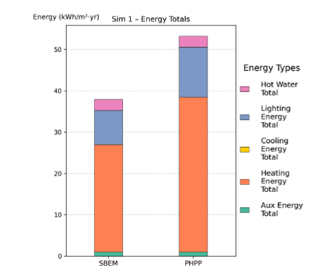
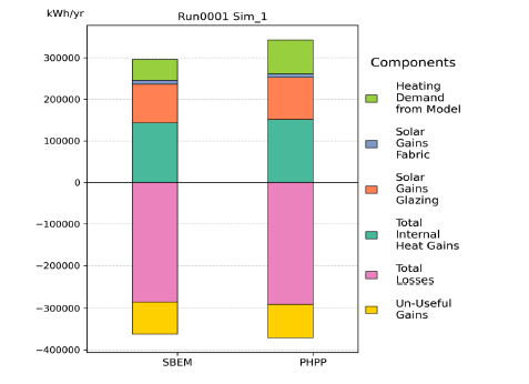
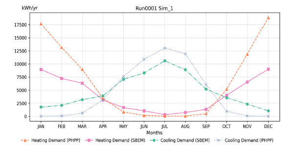
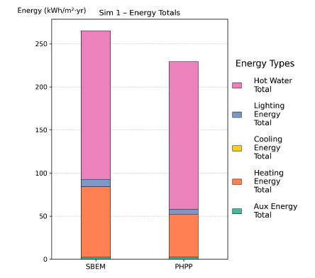
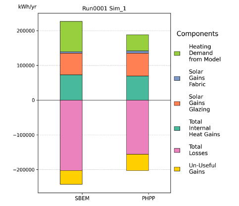
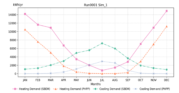
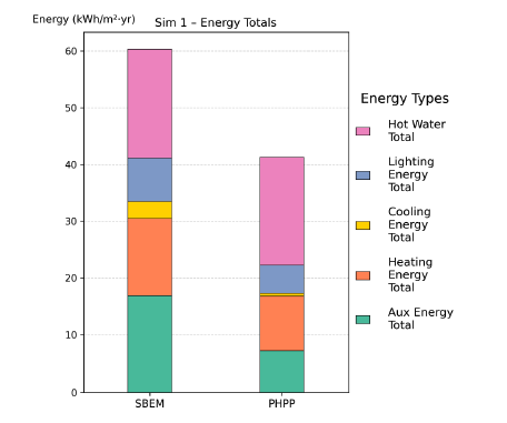
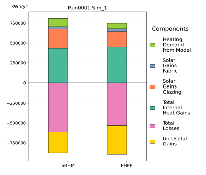
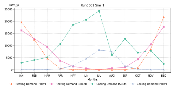
The energy balance for the models indicates that although the inputs have been aligned within both PHPP and SBEM the building physics calculations appear to drive some differences. For the three models considered gains for solar and internal sources aligned indicating the energy entering the condition zones was equal. The difference in losses are expected to be driven by the differences in zoning and granularity in which set points are applied. For example, the shallow-plan office is approximately the same, indicating that the whole building internal set point and operational hours for that set point align. For the secondary school and hotel it appears that the complexity of the model zones and the operational profile start to drive differences in the average set point, which in turn impacts loss rates as the building is on average at a lower or higher temperature. The most obvious example of this misalignment is present in the monthly cooling demand profile for the secondary school which shows a large drop in demand during the summer holidays. PHPP is unable to determine which month this drop will occur and models the annual average over a monthly profile.

A further difference that is driven by the misalignment of set points and profiles that the set point applied is the un-useful gains proport and therefore the heating demands and where present the cooling demand, where PHPP predicts a higher proportion of un-useful gains and a lower heating demand. The monthly demand data further evidences the lower heating demand in PHPP. It also demonstrates that cooling demand is also lower.

2.4.4 Discussion

There are many fundamental differences in the applied building physics algorithms, model standardisation and interpretation of input values between PHPP and SBEM. The results above outline the level of alignment that has been possible with PHPP using SBEM aligned input data (i.e. to minimise the differences in model standardisation and input data). Despite these efforts certain archetypes appear to have significant divergence on predicted key output metrics. The most notable are space heating and space cooling demand followed up auxiliary energy, which is partly sensitive to heating and cooling demands. If PHPP was to be populated with the intended conventions, differences in space heating and cooling are expected to be more significant. This is expected due to the following key differences in model function:

External dimensions

The total building heat transfer coefficient has been well aligned between SBEM and PHPP; however, if the external dimensions where applied, in line with PHPP conventions, and psi values adjusted to present the additional heat loss relative to the external boundary of building element connections, it is expected that PHPP would predict a higher heat loss rate than SBEM. Minor sensitivity testing indicated that no more than a 5% increase could be expected from the change in dimensions. The archetypes modelled in this study are simplistic in their geometry, should more complex buildings be compared then the differences in total heat loss may be significantly larger.

Window inputs

The granularity of window inputs is significantly higher in PHPP, with specific frame sections inputted as well as absorptivity and emissivity values for the frame. Furthermore, PHPP applies corrections for factors such as dirt as well as using an additional factor for incident solar reflection. The impacts of window overhang and side fin shading are more complex and account for the actual geometry of the shading object rather than the more simplistic approach from BS EN ISO 13790:2008 applied by SBEM.

Ventilated volume

PHPP assumes the ventilated volume based on conventions relating to space utilisation. This involves applying reduction factors to low use spaces such as cupboards and stairwells. This differs to SBEM where the entirety of the internal volume of the model is accounted for in ventilation and infiltration loss calculations. Furthermore, PHPP applies a different test method to SBEM where air leakage rates are required to be calculated with passive ventilators open. The PHPP model then allows for the useful ventilation volume within the calculations. SBEM, on the other hand, assumes that air leakage rates are exclusively through the fabric and no allowance is needed to be made for uncontrolled ventilation through passive ventilation devices.

Detailed system calculations

PHPP applies several detailed calculations to better predict the performance of heating, cooling, ventilation and lighting systems. In most cases these calculations are more detailed than those applied by SBEM, meaning that assessors need to have more information on the building for PHPP than SBEM.

The first key area relates to mechanical ventilation systems. Such systems are required to be input based on the system serving each unique zone in the model. These zones could be as small as individual rooms and the supply and extract rates for each zone are needed to be confirmed as well as ventilation system employed and the operational times for each zone. Each unique ventilation system requires physical characteristics to be entered, such as duct length, insulation and pressure losses. This significantly differs to the level of information needed for SBEM, which typically required the duct leakage rates to be declared as well as the specific fan power for each ventilation unit. This difference will result in modelled performance factors more representative to actual in use performance, which is typically much poor than predicted in SBEM. This more detailed approach in PHPP also applies to distribution pipework. SBEM has standard allowances for space heating and cooling distribution losses. Some more detailed inputs are required for SBEM’s modelling of hot water distribution and storage losses; however, these are less detailed than PHPP. The key additional areas of input data required by PHPP include distribution and stub/individual pipework diameters, insulation thickness, insulation conductivities, number tapping points, flow temperatures and circulation times. The result of this extra detail is often that PHPP hot water demands are higher than predicted in SBEM. The same is also true for heating and cooling system distribution; however, PHPP does calculate a usefulness factor for such losses, meaning that some of this energy displaces demand.

Occupancy, light, equipment and internal heat gains

For occupancy rates, the energy consumption associated with this occupancy and heat gains arising from this consumption, PHPP has several recognised assumptions that can be used. Unique activities in the building are captured and required lighting level, occupant density and schedules of usage are required. These PHPP default assumptions for typical activities within non-domestic buildings are available; however, for certification, evidencable assumptions on building use can be employed in the model, as is encouraged by CIBSE TM54. It should be noted that the NCM assumptions are not considered to be an alternative assumption set for PHPP. This study aligned the NCM database assumptions with the PHPP inputs for comparative purposes; therefore, it may not be considered a reasonable assumption for a certifiable assessment. Calculations within PHPP set the rate of heat gain from certain end uses (e.g. sensible heat gain from people performing typical activities) as well as the availability rates of gains (i.e. the percentage of energy consumption that is physically converted into heat).

These granular calculations are utilised to obtain an average heat gain rate for the heating and cooling seasons. For certification it is usually required that the PHPP default gain rate of 3.5W/m² is applied for the heating calculations, which can be significantly lower than the gain rates from the NCM. The result of this is substantially higher space heating demands and loads are predicted; meaning that more passive demand reduction measures (i.e. improved airtightness or insulation) are required to comply.

PHPP has a broader approach to equipment energy being captured than SBEM; this may be understandable as SBEM considers such equipment to be out of scope of the compliance calculations (i.e. unregulated energy). The result is that achieving the energy consumption metrics in PHPP are harder as many uses not captured by the NCM are included (lifts for example).

Daylighting utilisation calculations

In addition to the lighting level assumptions and schedules in PHPP, the model also requires room dimensions to be declared along with any associated glazing. Additionally, the glazing characteristics (i.e. light transmittance) are considered. This calculation module estimates the lighting level that can be feasibly met by daylight, reducing reliance on artificial lighting. SBEM has a similar calculation; however, the details of room geometries are less complex meaning the daylighting levels are likely to be less reflective of real-world levels.

Heating and cooling efficiency calculations

The detailed inputs for heating and cooling systems in PHPP follow ISO EN BS14825 test data format to confirm heating and cooling system performance at different loads and environmental conditions. PHPP can utilise this information to calculate SCOP and SEERs based on the declared system configuration (i.e. weather for the specific location, load ratio to demand, design flow temperatures). This differs to the approach allowed within SBEM where heating and cooling system efficiencies can be entered as a single static seasonal value. Typically based on the EN14511 standard and available on product datasheets, these figures are considered to be less accurate as they do not account for the specifics of the system (i.e. they are based on test rigs for standardised internal and external conditions). This particular element of PHPP is one of a number of examples where PHPP is considered a design tool, indicating if the proposed configuration is expected to deliver acceptable internal conditions.

Number of thermally independent zones

Arguably the most fundamental difference in building physics between PHPP and SBEM is the fact that PHPP creates a single thermally controlled zone, whereas SBEM can have multiple. For non-domestic^[1] buildings this can drive a large difference in the building physics between the models. In the case of this study, it is expected that much of the differences in predicted heating and cooling demands between PHPP and SBEM come down to the difference in model zones. Due to the single zone approach in large more complex buildings, PHPP is unable to predict localised cooling demand in response to small highly exposed zones (e.g. south facing meetings rooms). In SBEM, such zones would rapidly increase in temperature to above the set point, triggering cooling demand. In PHPP, the single zone has significantly more inertia meaning that solar gains can be absorbed throughout the building and cooling set points are not reached. Efforts were made with PHPPv10 to better predict overheating risk. For small buildings, such as dwellings, this additional module is understood provide improved understanding of overheating risk and therefore cooling. For large complex non-domestic buildings cooling demand prediction is still likely to be challenging with a single zone model.

A similar effect is present for heating; however, this is likely to be less significant for new non-domestic buildings as fabric standards and air tightness would result in fewer losses occurring in exposed zones relative to solar gains.

Renewables

PHPP has a more detailed set of inputs for the calculation of renewable energy generation technologies. This study has only sought to compare the photovoltaic array generation of buildings. The additional detail required by PHPP is used to calculate an array kWp, per orientation, pitch and shading condition. This is broadly similar to the inputs for SBEM. Monthly irradiance data is applied to obtain annual generation for each unique part of the array in both models. In SBEM inverter efficiency is assumed, whereas in PHPP this is a user input. Differences in weather data are more likely to be the driver of differences between PHPP and SBEM predicted solar yields.

Weather file

PHPP’s Glasgow Airport weather file was compared to the average monthly data produced for CIBSE TRY 2016 files for Glasgow. This indicated that there are differences in the monthly average temperatures and wind speeds across most months. This will drive differences in space heating and space cooling demand.

Summary

PHPP and SBEM differ both in terms of the modelling conventions and the underlying building physics calculations. Many of the differences in convention have been overridden/aligned for the purposes of this study. Despite this alignment, there are still significant differences between predictions of key regulated energy consumption rates (i.e. heating, cooling and auxiliary). By introducing more of the intended PHPP conventions, assumptions and standardisations this difference is expected to further increase, making SBEM and PHPP less comparable. Certain differences, such as the size and number of zones a building has could lead to irregular relationships between PHPP and SBEM.

It is important to note that PHPP is a more robust and potentially more accurate calculation methodology in many areas, particularly around system performance and granular reporting of expected building activities. Therefore, if applied in its own right (i.e. to achieve the PH standards for space heating demand, space cooling demand and primary consumption) PHPP is likely to drive a high standard of design and less likely to experience performance gap in real-world operation of buildings. To achieve the regulatory aim of conserving fuel and power it is possible the PHPP model, populated and validated by the Passivhaus Institute, through an accredited certifier, would likely achieve regulatory targets.

The use of PHPP as a regulation compliance tool would need to be carefully considered in light of the findings of this study. The sensitivity to building size and complexity and the irregular performance relative to SBEM indicates that the use of PHPP may need to be subject to specific use classes. There are many well documented non-domestic building typologies that have been certified by the PHI using PHPP. These include, offices, student accommodation buildings, schools and some healthcare and laboratory buildings. The PH standard promotes low energy design, particularly for space heating and cooling. In many cases it is likely that the PH certified building will meet or better the performance standards being considered in this study; however, it cannot be guaranteed that all non-domestic building types will comply if assessed through the SBEM notional building approach. Therefore, Scottish Government should consider for certain use types an alternative route for compliance may achieve regulatory aims.

2.4.5 Weather Sensitivity

PHPP version 10.6 contains a number of unique weather zones to support accurate modelling of demands. For Scotland there are a total of 9 weather zones, with a total of 14 weather files available. Within certain zones, multiple weather files are available to represent different levels of exposure and altitude. Weather data can be corrected from the altitude of weather station to the actual altitude of the building being modelled.

To understand the impact that varying weather files can have on key energy demands, PHPP variants analysis has been undertaken using four key weather files. The weather file tested include Glasgow airport (base case), Inverness (northern Scotland), Lerwick (island) and Carlise (representing southern Scotland). The below graphs display the most significant differences observed across the archetypes for space heating demand, heating load and space cooling demand.

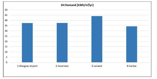
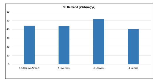
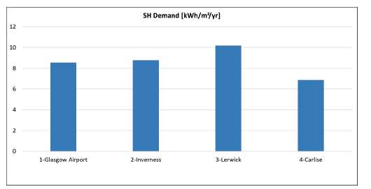
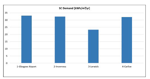
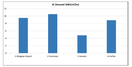
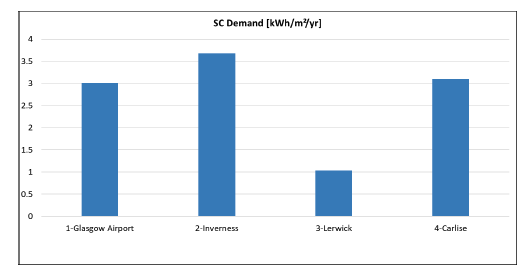
Across all building types, Lerwick consistently shows the highest heating demand, while Carlisle has the lowest. This consistent pattern suggests that climate and local weather conditions are strong drivers of heating energy needs, regardless of building type. Inverness and Glasgow Airport and Carlise display similar heating demand values within each building category, indicating comparable climatic conditions or building performance levels in these regions. Lerwick, in every case, stands out as the highest-demand location, due to the lowest average dry bulb temperatures and lower average solar irradiance. The relative demand between locations remains consistent across all three building types (hotels, schools, and office) despite significant differences the servicing strategy. While heating demand magnitude varies widely by building function (highest in hotels, lowest in schools), the geographic trend remains stable, reinforcing that location-specific factors influence all building types similarly.

For cooling demand, Inverness has the highest demand, suggesting a slightly greater need for indoor air conditioning or moisture control in the secondary school and hotel. For the shallow-plan office Inverness, did not have the highest cooling demand. This appears to be down to the higher glazing ratio of the building meaning the relatively higher solar irradiance levels in Glasgow Airport and Carlisle result in cooling demands greater than Inverness. Lerwick consistently shows the lowest cooling and dehumidification demand, due to the lower dry bulb temperatures and solar irradiance. Despite the relatively small values of cooling energy compared to heating, the consistency across all graphs highlights a clear climatic influence.