Small Business Bonus Scheme: evaluation
This report presents the results of an evaluation of the Small Business Bonus Scheme (SBBS), and provides recommendations in relation to the SBBS and non-domestic rates relief more broadly.
7 Econometric analysis
The analysis of Sections 4-6 was descriptive in nature. That is, for all the reasons we have described up to this point, it was primarily concerned with analysing broad trends in the NDR and survey data, and high-level comparisons across the distribution of RV. This is valuable for gaining an understanding of, for example, general features of the non-domestic property base and its interaction with the policy.
However, in evaluating a policy such as the SBBS, we wanted to obtain an estimate of its effect, on average, on the key business outcomes (e.g. Gross Value Added (GVA)) of its recipient businesses. This would represent an estimate of the extent to which the policy benefits businesses that receive SBBS relief. This means estimating some form of Average Treatment Effect (ATE).
Intuitively, we sought to understand the difference in the outcome of a business "treated" by the policy (i.e., in receipt of SBBS relief), had it not received the policy (its counterfactual). This would represent the 'true' causal effect of the policy. This counterfactual cannot, by definition, be observed.
Instead we used a feature of the design of the SBBS to construct counterfactual outcomes for businesses that would act as proxies for their outcomes in the absence of the policy. In this section, we set out the methodology for doing so and the results of our analysis.
7.1 Methodology
Obtaining the true causal effect of SBBS relief would require us to compare businesses which currently receive 100% SBBS relief with counterfactual versions of themselves receiving 25%, or no, relief (and vice versa).
This is not possible given that we cannot observe businesses in both their actual and counterfactual state. Obtaining an estimate of an ATE requires that we construct suitable proxies for the respective counterfactual groups.
Like many policies, the design of the SBBS is such that the characteristics of businesses that determines their eligibility for relief also determines how comparable they are. For example, the group of businesses in receipt of 25% SBBS relief do not serve as an appropriate counterfactual for the group of businesses in receipt of 100% relief. Using them as such would mean comparing businesses with RVs of between £1 and £15,000 with those whose RV is between £15,001 and £18,000; a comparison that is uninformative given the average business that operates in premises valued between £1 and £15,000 (and which receives 100% relief) is likely to be considerably different to the average business operating from premises valued between £15,001 and £18,000 (which receives 25% relief). This makes it impossible to isolate the true effect of receiving 100% relief compared to 25% relief.
At the same time, however, the cliff-edge in relief around well-defined RV thresholds (for single-site businesses) does allow us to focus on a group of businesses that should provide suitable comparators for one another.[42] That is, again using the 100% threshold as an example, we would expect that, on average, a business with an RV of £14,999 is comparable to a business with an RV of £15,001 except for the level of SBBS relief they receive. If this is the case, comparing the outcomes of the businesses immediately on either side of this cut-off would provide an estimate of the average effect of receiving 100% versus 25% relief at the margin. This logic extends to a comparison of businesses with an RV of £17,999 and £18,001, the RV threshold at which SBBS relief falls from 25% to zero.[43]
Formally, assume yis represents the business outcome for each business i in state of the world s. Here i simply indexes businesses from 1 to N, N, being the total number of businesses, and s indicates whether a business receives 25% (s = 0) or 100% (s = 1) relief. We focus on this comparison here for simplicity. Given our description above, we can define the ATE as:[44]
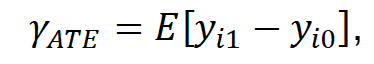
(1)
This is the (unobtainable) average difference in outcomes of business with and without 100% relief – note both the left and right y have a subscript i, indicating they represent the outcome of the same person. If 100% and 25% SBBS relief were randomly assigned to businesses, a simple comparison of outcomes between the two groups would be enough, giving:
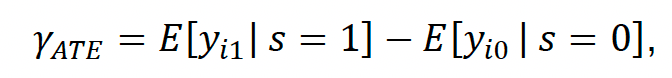
(2)
where the right-most expression acts as a substitute for E[yi0 | s = 1]– the outcome of business when in receipt of 25% relief (yi0), given that they have in reality been awarded 100% relief (s = 1).
However, SBBS relief is not awarded randomly; rather, it is a function of the RV of each business's properties. As a result, the outcome (yi) is not independent of the relief level a business receives. Again, due to the design of the SBBS we know the rules that determine this dependence. In the notation of equations 1 and 2, we know that:
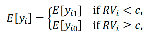
(3)
where c represents the threshold value, which, under the current policy, is £15,001. Put simply, we know the level of relief a business is eligible for is based solely on the RV of its properties. Given that we are focusing on the example of comparing 100% and 25% recipients, we assume here that £18,000 is the maximum RV of a business.
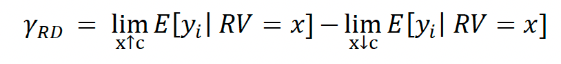
When RV is very close to the threshold (c), businesses arguably become increasingly similar. We can exploit this fact to define another treatment effect, the regression discontinuity (RD) treatment effect, which is given by:
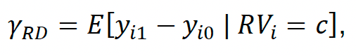
(4)
This effect differs from yATE in that it is local, meaning it represents the average effect on their outcome for businesses with an RV equal to (£15,001) if the level of relief they received were switched from 25% to 100%. It therefore does not tell us anything about how businesses with an RV that falls far away from the threshold are affected by the policy. Again, as with everything we outline here, the same logic applies to the effect at the 25% SBBS threshold (where RV is £18,001).
If the thresholds are exogenously defined the above expression is equivalent to
(5)
Further, if the two expectations that make up this difference are continuous, then we can calculate yRD as
(6)
In words: the RD treatment effect is equivalent to the limit of the expectation functions either side of the threshold given that they are continuous (note the omission of the s subscript on each y).
Intuitively, extremely (in fact, infinitesimally) close to the cutoff the average outcome among businesses with an RV just above the threshold (those in receipt of 25% relief) should provide a suitable counterfactual for those businesses with an RV just below the threshold (and thus in receipt of 100% relief). With no other systematic differences between these two groups, other than their eligibility and receipt of SBBS relief, we attribute differences between them to the effect of the policy.
There are four principal assumptions underpinning this approach to estimating the effect of SBBS relief on its recipients. They are that:
1. the treatment is a deterministic function of RV – the assignment variable;
2. there is a discontinuity in the level of treatment at a known value of the RV – the threshold;
3. RV cannot be manipulated to influence whether or not businesses receive SBBS relief; and
4. other 'control' variables do not change discontinuously at the threshold.
Assumptions 1 and 2 are satisfied given that the thresholds for RV are well defined. Assumptions 3 and 4 are both concerned with the comparability of individuals on either side of the threshold. For instance, concerning Assumption 4, if for some reason it were more likely that particular types of properties, e.g. shops, had an RV just below the threshold while otherwise equivalent, e.g. industrial, properties were more likely to have an RV just above the threshold, and shops on average benefit more from the SBBS than industrial properties then the "treatment" and "control" groups are endogenously determined and any estimate of yRD would overestimate the effect of the SBBS. We haven't found any evidence of this in the data.
In terms of Assumption 3, there is some evidence of bunching in the RV distribution just below the £15,000 RV threshold that has appeared in the NDR data since this RV threshold became a feature of the policy (see Figure 4.13). This suggests that, after the point in time at which an RV of £15,000 became a threshold determining whether a business receives 100% relief or 25% relief, a higher proportion of businesses were attributed an RV just below £15,000.
If the likelihood of being placed below the threshold is endogenous to business outcomes, Assumption 3 will be violated and any estimates of the effect of the policy will be biased. For example, if the likelihood of being placed just below the threshold is correlated with business need for NDR relief[45], and business need is correlated with business outcomes, comparing the outcomes of businesses just below the threshold (which have a higher need and on average worse outcomes) with those above (which have less need and on average better outcomes) will under-estimate the effect of the SBBS. If this bunching persists in the data we use here, we need to be cognisant of the presence of potential biases (both negative, as we have illustrated here, but potentially positive, as we have no information on the source of the bunching; it could be, for example, that well-managed businesses are more likely to appeal) when drawing conclusions from our analysis.
As an example of what we might expect in a neat (and artificial) example of a discontinuity, Figure 7.1 plots simulated values of GVA data across the RV distribution. Each gray dot represents the average GVA within £500 RV groups, and the black line a line that best fits the relationship between RV and GVA. From this we might infer from the discontinuous drop in the best-fitting line at the 100% SBBS threshold that the SBBS positively affects businesses' value added. If receiving 100% relief has any such effect, for example through increasing re-investment or innovation in recipient businesses, then we would expect similar discontinuities to appear when we plot data on actual outcomes across the RV distribution. We examine these types of plot using the available data for Scotland across several outcomes in Section 7.4.
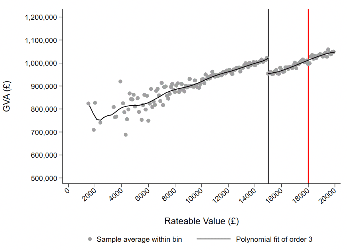
Note: the data used to generate this figure are simulated. The black vertical line represents the 100% SBBS threshold and the red vertical line the 25% threshold. For illustrative purposes, the graph has been produced assuming no effect at the 25% threshold.
7.2 Data matching and sample construction
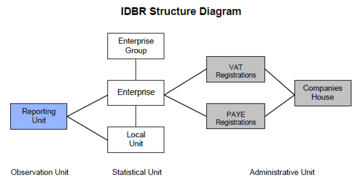
The Scottish Government matched properties in the 2018 Billing Snapshot and Valuation Roll to enterprises in the Interdepartmental Business Register (IDBR) – an administrative record of all enterprises, as they are referred to in the IDBR, in the UK that are VAT registered and/or operate a PAYE scheme. Each enterprise in the IDBR has a unique reference number that uniquely identifies it from all others in the UK. These enterprises can be part of a wider enterprise group, or comprise smaller local units (Figure 7.2).
In total there were 130,861 properties used in the matching exercise, representing 86% of all SBBS recipients. An implication of the criteria for inclusion in the IDBR (i.e. being VAT registered – which requires a turnover of at least £80,000 – and/or operating a PAYE scheme) is that it does not contain information on extremely small businesses. Because of this, the Scottish Government excluded property types that were not likely to be found in the IDBR – such as public toilets and sewerage tanks – and those categories with less than 100 SBBS recipients. Still, it is important to note that for a business to be successfully matched to a record in the IDBR it must meet these criteria, as it affects the composition of the eventual post-matching sample. The Scottish Government produced a matching report which provided more detail on the property types excluded from the matching exercise (see Appendix F).
Of these 130,861 properties, 70,819 (54%) were matched to an enterprise in the IDBR. All properties for which this exercise was successful were linked to only one enterprise in the IDBR. However, 8,917 (12.6%) of these matches were to an enterprise that had ceased trading prior to January 1st, 2017. As a result, only 61,902 (47.3%) of the 130,861 properties were successfully matched to a viable enterprise in the IDBR. Again, although we cannot know with any degree of certainty, it is likely that a portion of the 46% properties not matched to an IDBR record did not meet the criteria for inclusion.
This means the 61,902 properties represent a sample of enterprises that are VAT-registered and/or operating a PAYE scheme, a fact that must be borne in mind when we come to define the effect of SBBS relief we seek to estimate. The Scottish Government's matching report (included in Appendix F) provides a full description of the method used to match properties in the VR to enterprises in the IDBR, as well as a breakdown of the class (a classification of property type), core (another classification of property type), RV and location of matched properties.
Source: BSD User guide
The aim of this matching exercise was to retrieve unique reference numbers with which properties from the Valuation Roll could be linked to information in administrative data on business outcomes such as turnover, employment and GVA. Figure 7.3 below shows how the three datasets are connected.
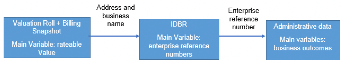
A shortcoming of matching to enterprises in this way is that we are not able to retrieve lower-level information on business outcomes; for example, associated only with activity in Scotland or for specific locations (enterprises might have other locations outside or within Scotland). This might affect estimates of the effects of the SBBS if, for example, its benefits are mainly experienced at the local unit level (Figure 7.2). Given that we are eventually using information aggregated to the enterprise level, these effects might be lost in amongst any other changes taking place across other local units. Unfortunately, this is unavoidable.
The validity of any inference from an econometric analysis of the SBBS using these data is in large part determined by the accuracy of the matches between properties and enterprises. The matching was carried out based on business name and address information, in a similar fashion to the categorising of properties into businesses outlined in Section 3.2 (although this relied solely on business name).
The Scottish Government's matching report outlined this process in detail as well as how the quality of matches was determined. Appendix D outlines in detail how we used data made available for this portion of the evaluation to assess the feasibility of matching in this way based on differences in the categorization of businesses into groups in the IDBR (enterprises) and the VR (businesses).
Although properties were matched to only one enterprise, the reverse was not true. This meant we could classify properties in two different ways pre- and post-matching. Pre-matching, as has been the case throughout this report, prior to being matched properties were classified as being single-site or multi-site businesses based on Scottish Government estimates (See Section 3.2). Post-matching, we can make a similar categorisation to classify properties as being part of either a single- or multi-property enterprise based on their match to enterprises. As a result, we were able to compare these two and evaluate their consistency in terms of the site count and the implied cumulative RV.
For example, say a property with an RV of £5,000 was grouped together with six others in the VR with the same RV. This would categorise it as being in a multi-property business with a site count of 7 and a (hypothetical) cumulative RV of £35,000. However, when matching these properties to the IDBR, they may not all be attributed to the same enterprise, leaving the enterprise with a lower cumulative RV than in the VR. For example, if only one were not matched, the enterprise would incorrectly be classed as having six properties and a cumulative RV of £30,000. The non-matched site would also be incorrectly classed as a single-site, single-property enterprise with an RV of £5,000. Moreover, it may be the case that other (unrelated) properties are attributed to this enterprise.
In a perfect matching scenario, all properties that are categorised as of single-site businesses in the VR would be the only properties matched to an enterprise in the IDBR. Similarly, all properties estimated to be part of a multi-site businesses would match to the same IDBR enterprise. This would mean site counts and RVs would be consistent across enterprises, and suggest that the Scottish Government's business groupings and matching were accurate. There are a number of reasons why, despite the best efforts being made to accurately link these data, this might not be the case.
The estimates of business groupings could be inaccurate, as could be the matching of businesses in the VR to IDBR enterprises. It is also the case that both could be incorrect. An additional complication stems from the IDBR matching procedure: given the requirements for inclusion, businesses deemed to be unlikely to match to an enterprise in the IDBR were excluded, meaning that property counts and RVs might differ within enterprises because part of their business has been removed.
Appendix D – where we aim to understand the extent to which this might have occurred – compares the site count of matches in more detail, and outlines how we define consistency within multi-property enterprises. We primarily rely on 'businesses/enterprises' site count to evaluate the consistency of matches given that it is the most straightforward way to categorise properties into the two groups for which the SBBS eligibility rules differ. Detail on how we define consistency is given at the end of Appendix D.
In short, the results of this analysis provide little evidence that there is consistency between business groupings in the VR and enterprise groupings in the IDBR matching. We also describe the implications of the apparent mismatch for total business RV and SBBS relief levels – business characteristics central to our analysis – and find that the inconsistencies in matching lead to large discrepancies in total RV and levels of relief within enterprises. As a result, it is unclear which value of each we should use for these businesses in our analysis. We do not have any way of fully identifying businesses in the Valuation Roll, and so we are unable to determine the extent to which these discrepancies are a result of inaccuracies in Scottish Government estimates of either business groupings in the Valuation Roll, or matches between the VR and enterprises in the IDBR.
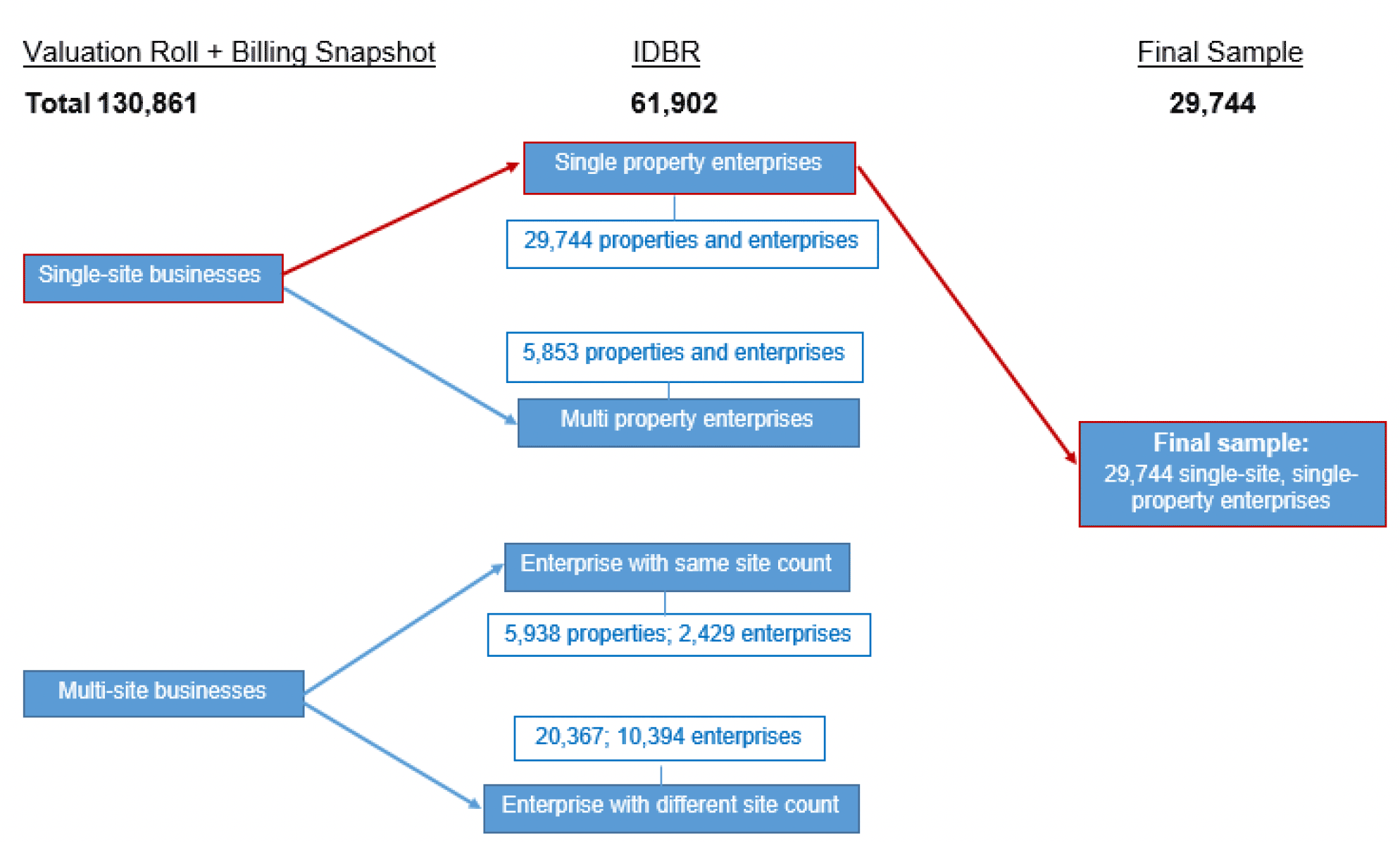
Due to these significant discrepancies, we limit the sample for this part of the evaluation to the 29,744 properties that were estimated to be a single-site business and were the only property matched to their enterprise in the IDBR. We call this restricted sample single-site, single-property enterprises. This is 69.7% of all enterprises and 48.1% of all properties used in the matching exercise. Figure 7.4 below shows, in the form of a flow diagram, how the overall sample of properties from the VR eventually reduces to the final sample of single-site, single-property enterprises.
The purpose of this – and indeed any – econometric analysis is to clearly define and estimate an effect of SBBS relief using a robust methodology. This is not possible if we cannot first define our sample and attribute the enterprises in the sample to outcome data with a reasonable degree of certainty. Restricting the sample to only single-site, single-property enterprises allows us to focus on a somewhat well-defined sample and reduces the likelihood – although not entirely – of using incorrect information on enterprises.[46] As a result, however, we can only attempt to estimate the effect, on average, of the SBBS on the marginal single-site, single-property enterprise that is VAT registered and/or operating a PAYE scheme, as opposed to the population-wide effect of SBBS relief at the threshold.[47]
7.3 Characteristics of the single-site, single-property enterprise sample
The decision to focus on this sub-sample reduces our sample to 29,744 enterprises/properties; 69.7%/48.1% of the full sample. Figure 7.5 shows the RV distribution of these enterprises. The mean RV in the sample is higher than that among the population of single-site businesses described in Section 4.1 (~£5,000). Comparing with Figure 4.2 this is because there are far fewer low-RV properties in this sample when compared with the population; an artefact of both the criteria for inclusion in the matching exercise and the likelihood that properties with a relatively higher RV were successfully matched.
The most notable feature of the distribution in Figure 7.5 is that there is substantial bunching around the SBBS thresholds: there is a significantly higher proportion of businesses immediately below both the 100% (£15,000) and 25% (£18,000) thresholds than above. As discussed, this bunching was a feature of the distribution of the entire population of properties, both in the recent and historical data.
The fact this bunching persists in the vastly reduced sample we have constructed for this portion of the evaluation ex ante compromises the validity of our econometric analysis. We set out in the preceding subsection that the absence of manipulation in the assignment variable (RV) is a necessary condition for using the regression discontinuity methodology to estimate an unbiased policy effect. As Figure 7.5 shows, however, this condition is not met.
If it were, there would be a (relatively) smooth decline in the height of the bars moving from left to right, with little sign of jumps in successive bars. Although we can still proceed with the analysis, we need to be aware of the bias this might imply when drawing conclusions. We also discussed, in Section 4.7, how some of this bunching is likely a result of a higher rate of appeals among those revalued just above the 100% threshold.
To illustrate this, Appendix Figure E.1 shows that the same bunching is not present in the distribution of draft RVs in the sample. Although this allows us to consider what the potential direction of the bias will be, we do not have enough information to determine this with any certainty. We describe later in this section some additional analysis we undertook using these draft RV data to understand whether they can shed any light on this.
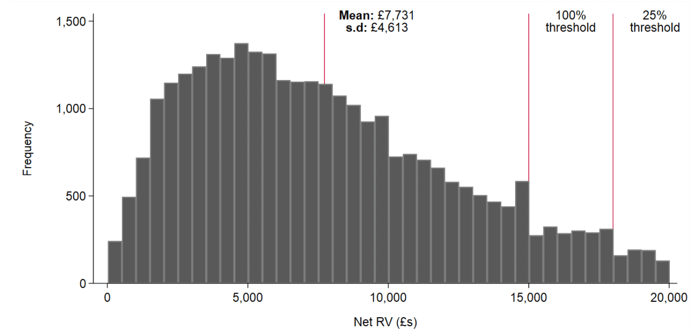
Note: Properties/enterprises are grouped into £500 RV bands. For example, the bar between 0-£500 groups all properties with an RV in the range.
Table 7.1 shows that the distribution of properties across classes (property types) in the sample is somewhat similar to that in the population but there are key differences: although not in precisely the same order, by far the most common classes of non-domestic property are shops, industrial subjects and offices. The prevalence of these classes of property in the sample are in fact more pronounced than in the population.
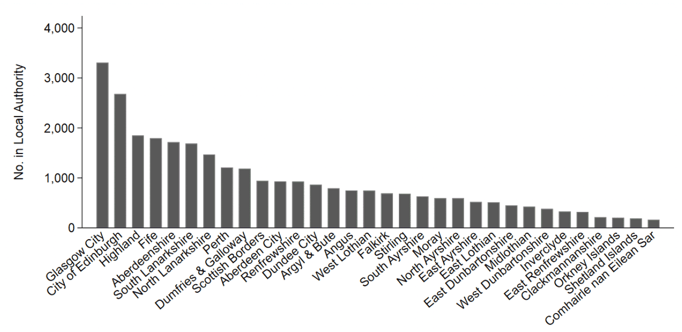
Figure 7.6 shows that the distribution of properties across local authorities in the sample is similar to that in the population as a whole. The two local authorities with the most properties/enterprises are the cities of Glasgow and Edinburgh, followed by Highland (the largest local authority by land mass), Fife and Aberdeenshire. In the population, Highland in fact has the second largest non-domestic property base ahead of Edinburgh City (see Section 4.1). In the sample, however, it accounts for a substantially lower proportion of enterprises, likely due to average RV being lower in Highland than in Scotland as a whole. As a result, and as with property classes, the dominance of the local authorities with the most properties is greater in the sample than in the population.
This suggests that the restricted sample of single-site, single-property enterprises differs from the wider population of non-domestic properties. It contains, on average, higher RV properties, a far larger proportion of shops, offices and industrial subjects, and properties that are more concentrated in two of Scotland's major cities, Edinburgh and Glasgow.
| Number of Enterprises/properties in the sample | Proportion of the Sample | Proportion of class among population of SBBS claimers | |
|---|---|---|---|
| Shops | 11,738 | 39.46 | 26.60 |
| Industrial Subjects | 8,185 | 27.52 | 22.73 |
| Offices | 5,229 | 17.58 | 13.43 |
| Leisure & Entertainment | 1,385 | 4.66 | 16.54 |
| Garages & Petrol Stations | 828 | 2.78 | 2.15 |
| Public Houses | 666 | 2.24 | 0.86 |
| Health & Medical | 633 | 2.13 | 1.01 |
| Hotels etc. | 555 | 1.87 | 3.03 |
| Other* | 122 | 0.41 | 2.84 |
| Public Service Subjects | 108 | 0.36 | 1.03 |
| Cultural | 107 | 0.36 | 0.26 |
| Care Facilities | 91 | 0.31 | 0.24 |
| Statutory Undertakings | 48 | 0.16 | 0.09 |
| Education & Training | 29 | 0.1 | 0.12 |
| Sporting Subjects | 20 | 0.07 | 8.91 |
| Total | 29,744 | 100 | 73.24 |
Note: * contains <10 properties used by religious organisations. The population column does not sum to 100 because five property classes are not represented in our sample: advertising, quarries & mines, petrochemical, communications. The proportions in this column are from column 2 of Table 4.3.
There are also a number of enterprises that are eligible for the SBBS but are recorded as receiving no relief, or which receive a relief level that differs to that which is suggested they should receive according to their RV. Table 7.2 below shows the number of matched enterprises by their claim status. In our main analysis we focus on SBBS claimers, and so omit enterprises with an RV below £18,000 that receive no relief or that do not receive either 100% or 25% relief.
| Claim status | Number | % |
|---|---|---|
| Eligible 100 % claimers | 25,022 | 84.13 |
| 100% claimers claiming less | 536 | 1.8 |
| Eligible 25% claimers | 1,418 | 4.77 |
| 25% claimers claiming less/more* | < 10 | . |
| Eligible non-claimers | 2,086 | 7.01 |
| Ineligible non-claimers | 672 | 2.26 |
| Ineligible claimers* | <10 | . |
Note: * These groups have fewer than 10 enterprises so cannot be reported separately for statistical disclosure reasons.
7.4 Linking the restricted sample to the ABS and BSD
The next step in the analysis required linking the restricted sample of enterprises to information on business outcomes. We were provided two administrative sources of data with which we could do so: the Business Structures Database (BSD) and a portion of the Annual Business Survey (ABS). The BSD contains information on business turnover, employment and location. The ABS contains more detailed data on businesses cost structure, and so provides estimates of GVA and total output. It only contains a sub-sample of businesses from the BSD, however, and disproportionately samples large (250+ employees) businesses.
We linked the matched sample of properties to the 2018 BSD using their unique enterprise reference number. Only 1,334 (4.7%) of the 29,744 enterprises in the restricted sample were not able to be linked to the BSD, 1,210 of which were recorded as receiving SBBS relief. Of these non-linked SBBS recipients, 1,150 (95%) received 100% relief. RV was similar on average among the linked and non-linked enterprises: for the former group the mean RV was £7,764, and for the latter it was £7,028. Table 7.3 below shows that these are distributed across RV levels in a similar manner as the linked enterprises. There were a higher proportion of shops and lower proportion of industrial subjects and offices in the matched enterprises that could not be successfully linked to the BSD.
We cannot know why these businesses were not found in the BSD, although it could result from misalignment between the dates at which the BSD snapshot was taken from the IDBR and the date at which the enterprises appeared within it – this could occur if an enterprise is newly created or crosses the VAT or PAYE threshold. Again, given the matching was carried out on addresses using the IDBR as at June 2019 but the Billing Snapshot is for 2018, there is also a chance that there are mismatches to enterprises that did not actually exist in 2018. As a check, we also attempted to link enterprises to the 2017 BSD. More than double the number of businesses could not be linked when using only the 2017 data, and allowing properties/enterprises to be matched to data in either 2017 or 2018 only results in an increase of 52 successful linkages.
Not all of the successful linkages were to enterprises registered in Scotland. Table 7.4 show that roughly 3.5% (1,197) were matched to enterprises in other regions of the UK. Some of the data made available to us allowed us to explicitly focus on economic activity in Scotland.
In the ABS data, instead of enterprise-level information, we were provided with data on all local units (see Figure 7.2) in Scotland over the years 2008-2018. To calculate enterprise level data from these, we totaled all the local unit information within each enterprise. Doing so for 2018 and linking the resulting data to the single-site, single-property enterprises results in 82.9% (24,661) of the 29,744 being successfully linked.
This is significantly lower than when matching to the BSD (95.3%), but in fact is still relatively high considering that the ABS contains only a subsample of businesses from the BSD. Allowing for enterprises to be linked in either 2017 or 2018 increases the success rate to 88.2% (26,223). This increase could be due to either differences in the sampling across years or business closures between 2017 and 2018. We focus on matching only in 2018 since this is the reference year for the NDR data.
| Max. RV in band | Not linked | Linked |
|---|---|---|
| 1,000 | 35 | 702 |
| 2,000 | 88 | 1,687 |
| 3,000 | 127 | 2,221 |
| 4,000 | 136 | 2,417 |
| 5,000 | 127 | 2,538 |
| 6,000 | 124 | 2,516 |
| 7,000 | 112 | 2,205 |
| 8,000 | 116 | 2,181 |
| 9,000 | 94 | 2,001 |
| 10,000 | 84 | 1,800 |
| 11,000 | 43 | 1,423 |
| 12,000 | 58 | 1,311 |
| 13,000 | 52 | 1,081 |
| 14,000 | 29 | 944 |
| 15,000 | 40 | 986 |
| 16,000 | 19 | 581 |
| 17,000 | 22 | 567 |
| 18,000-20,000* | 28 | 1,249 |
| Total | 1,334 | 28,410 |
Note: * some categories in this group contain fewer than 10 observations among the linked enterprises. Numbers cannot be reported for statistical disclosure reasons.
| Region | Number | % |
|---|---|---|
| East | 95 | 0.33 |
| East Midlands | 72 | 0.25 |
| London | 206 | 0.73 |
| North East | 58 | 0.2 |
| North West | 138 | 0.49 |
| Northern Ireland | 32 | 0.11 |
| Scotland | 27,398 | 96.49 |
| South East | 156 | 0.55 |
| South West | 77 | 0.27 |
| West Midlands | 71 | 0.25 |
| Yorkshire and The Humber | 91 | 0.32 |
| Total | 28,394 | 100 |
7.5 Characteristics of the sample linked to the BSD
We first look at the composition of the linked sample relative to the wider population of businesses in Scotland. Table 7.5 shows how linked enterprises (column 2) compare to the wider population of enterprises in Scotland (column 1). Overall, the linked enterprises from the NDR data have more employees, higher turnover and are more likely to be in retail, accommodation and food or other services than the wider enterprise base. This comparison does not tell us how SBBS recipients differ, on average, from the wider population of enterprises, but simply reflects that the process by which the final sample of businesses was constructed changes the characteristics of the sample a little.
Table 7.5 shows that there is substantial variation in turnover and employment within the sample. To see how these two outcomes vary within RV groups – which will define our comparison groups – Table 7.6 shows the mean and standard deviation of income within each of the 18 different £1,000 RV bands below £18,000, both for the full sample, and for SBBS recipients only. In its first two columns, it shows two striking features of the samples within RV groups.
The first two columns refer to the full sample of single-site, single-property enterprises. The variation in turnover and employment is enormous within all RV bands. Further, both the mean and variation in turnover are by far the largest in the £1,000 band immediately below the 100% threshold. The second two columns consider only SBBS recipients and show that this variation below the threshold is reduced when excluding enterprises that are eligible but not recorded as receiving SBBS relief. There is a similar effect across the majority of the RV bands in the last two columns of Table 7.6. Given that the focus of this section of the evaluation is estimating the effect of the SBBS on claimers, it is this sample that we use for the analysis which follows.[48]
Together Tables 7.5 and 7.6 suggest two things. First, businesses vary substantially in terms of turnover and employment even when conditioning on RV – the variation in turnover and employment within the RV bands is much larger than the variation in averages between RV bands – which brings into question whether RV is a good measure of business size, and by extension their need for business support.[49]
The SBBS is predicated on aligning support to business need – specifically that small businesses might require help paying their non-domestic rates in order to launch, operate, and grow. Although not a perfect indicator, turnover and employment can act as rough proxies for business activity, and perhaps 'need'. We have shown that businesses in narrow £1,000 RV groupings vary greatly in terms of these measures suggesting that although they are similar in terms of their RV, they are highly dissimilar in terms of business activity.
| (1) All Scottish enterprises in the BSD | (2) Single-site, single-property enterprises linked to the BSD | |
|---|---|---|
| Mean turnover (£000s) | 1,495 | 4,781 |
| (104,929) | (308,137) | |
| Mean no. of Employees | 10 | 20 |
| (292) | (490) | |
| Employees banded (proportions) | ||
| 0-9 | 0.91 | 0.86 |
| [195,710] | [24,300] | |
| 10-49 | 0.07 | 0.12 |
| [15,392] | [3,462] | |
| 50-99 | 0.01 | 0.01 |
| [1,841] | [288] | |
| 250+ | 0.00 | 0.01 |
| [997] | [184] | |
| Turnover banded (proportions) | ||
| <£50,000 | 0.28 | 0.07 |
| [59,306] | [2,056] | |
| £50,000-£99,999 | 0.22 | 0.17 |
| [46,539] | [4,881] | |
| £100,000-£249,999 | 0.29 | 0.37 |
| [61,245] | [10,427] | |
| £250,000-£499,999 | 0.10 | 0.19 |
| [21,330] | [5,455] | |
| £500,000-£999,999 | 0.05 | 0.10 |
| [11,736] | [2,888] | |
| £1,000,000-£1,999,999 | 0.03 | 0.05 |
| [6,507] | [1,300] | |
| >£2,000,000 | 0.04 | 0.05 |
| [7,979] | [1,403] | |
| Industry (proportions) | ||
| A: Agriculture, Forestry & Fishing | 0.09 | 0.03 |
| [18,802] | [834] | |
| B: Mining and Quarrying | 0.00 | 0.00 |
| [352] | [12] | |
| C: Manufacturing | 0.05 | 0.07 |
| [11,225] | [1,962] | |
| D: Electricity, Gas, Steam & Air Con. | 0.00 | 0.00 |
| [840] | [69] | |
| E: Water Supply, Sewerage, Waste | 0.00 | 0.00 |
| [511] | [78] | |
| F: Construction | 0.11 | 0.09 |
| [23,992] | [2,622] | |
| G: Wholesale & Retail | 0.17 | 0.27 |
| [36,248] | [7,739] | |
| H: Transportation & Storage | 0.03 | 0.02 |
| [6,473] | [706] | |
| I: Accommodation & Food Services | 0.07 | 0.15 |
| [14,092] | [4,177] | |
| J: Info. & Communication | 0.06 | 0.02 |
| [12,733] | [539] | |
| K: Financial & Insurance | 0.02 | 0.01 |
| [3,689] | [362] | |
| L: Real Estate | 0.04 | 0.02 |
| [8,066] | [651] | |
| M: Professional, Scientific, Technical | 0.18 | 0.09 |
| [38,585] | [2,488] | |
| N: Admin. & Support | 0.08 | 0.05 |
| [16,414] | [1,488] | |
| P: Education | 0.01 | 0.01 |
| [2,182] | [217] | |
| Q: Human Health & Social Work | 0.03 | 0.04 |
| [6,676] | [1,062] | |
| R: Arts & Entertainment | 0.02 | 0.02 |
| [4,147] | [434] | |
| S: Other Services | 0.04 | 0.10 |
| [7,522] | [2,959] | |
| O, T, U: Public Admin. & Defence, Activities of Households, Extraterritorial Organisations* | 0.01 [2,093] | 0.00 [11] |
| N | 214,642 | 28,410 |
Note: Numbers are averages. For turnover bands, employee bands and industry this represents the proportion in each. Square brackets contain counts, parentheses contain standard deviations. * all 3 categories contain < 10 observations so have been combined.
| Full sample of single-site single-property enterprises | SBBS recipients only | |||
|---|---|---|---|---|
| Max. RV in band | Turnover | Employment | Turnover | Employment |
| £1,000 | 24,122 | 59 | 26,509 | 52 |
| (614,091) | (1,190) | (653,373) | (1,239) | |
| £2,000 | 3,648 | 29 | 890 | 5 |
| (73,551) | (576) | (10,621) | (23) | |
| £3,000 | 1,508 | 12 | 830 | 7 |
| (24,438) | (124) | (17,729) | (87) | |
| £4,000 | 2,127 | 15 | 783 | 7 |
| (47,270) | (324) | (10,890) | (112) | |
| £5,000 | 1,504 | 18 | 644 | 9 |
| (24,279) | (278) | (9,053) | (178) | |
| £6,000 | 1,009 | 9 | 727 | 7 |
| (10,327) | (73) | (8,186) | (59) | |
| £7,000 | 1,509 | 12 | 1,002 | 9 |
| (16,721) | (172) | (12,099) | (169) | |
| £8,000 | 2,243 | 11 | 1,755 | 6 |
| (52,250) | (106) | (52,080) | (44) | |
| £9,000 | 1,766 | 20 | 1,566 | 19 |
| (29,533) | (406) | (29,651) | (416) | |
| £10,000 | 1,253 | 14 | 678 | 9 |
| (10,279) | (114) | (3,915) | (62) | |
| £11,000 | 6,591 | 13 | 6,219 | 8 |
| (199,243) | (105) | (205,341) | (43) | |
| £12,000 | 1,550 | 15 | 814 | 10 |
| (13,366) | (94) | (6,617) | (59) | |
| £13,000 | 2,386 | 16 | 902 | 10 |
| (29,228) | (126) | (5,592) | (68) | |
| £14,000 | 4,749 | 77 | 2,052 | 10 |
| (71,957) | (1,952) | (36,542) | (62) | |
| £15,000 | 49,871 | 17 | 723 | 10 |
| (1,526,805) | (151) | (2,742) | (42) | |
| £16,000 | 3,871 | 36 | 3,384 | 34 |
| (31,959) | (237) | (33,937) | (252) | |
| £17,000 | 4,276 | 38 | 1,192 | 13 |
| (31,712) | (358) | (6,215) | (54) | |
| £18,000 | 12,717 | 19 | 717 | 9 |
| (271,351) | (143) | (1,922) | (12) | |
Note: The 'Max. RV' represents the maximum RV within each band, where each band starts immediately above the maximum of that which precedes it. Numbers are means, standard deviation are in parentheses. For columns 1 and 2, corresponding counts within RV bands are in Table 7.3. For columns 3 and 4, numbers are 642, 1,592, 2,153, 2,356, 2,487, 2,487, 2,194, 2,140, 1,946, 1,731, 1,327, 1,216, 992, 860, 899, 487, 465, and 466 for the 18 categories respectively.
Second, they provide further evidence that there is endogenous bunching into the RV band just below the £15,000 threshold for 100% relief based on business need: focusing on SBBS recipients, as RV increases there is a general upward trend in turnover, except for a notable drop in the band just below the threshold and a notable increase in the band above the threshold. This suggests that it tends to be smaller businesses that are being 'sorted' below the threshold.
The large variability in outcomes across the assignment variable (RV) means that estimates of the effect of the SBBS at the threshold are likely to be imprecise. Moreover, as we have noted, the sorting of businesses below the threshold means any estimate of the effect of additional relief will be biased. In our analysis of the effect of SBBS relief that follows, we have primarily focused on all businesses that receive SBBS relief in the sample of single-site, single-property enterprises. Given that there are only a small number of such enterprises above an RV of £18,000, we also focus our analysis on the threshold where relief drops from 100% to 25%. The sample sizes within RV bands around this threshold in which we might assume businesses are comparable are already relatively small (986 in the £1,000 below £15,000 and 581 in the £1,000 band above).
If we focus on one particular type of business, for example shops, we restrict the sample size even further. The potential benefit of doing so is to reduce variability in outcomes and make estimates more precise, but a reduction in variability is not guaranteed for two reasons: the reduced sample size from restricting the sample, and the fact that businesses operating from shops are also diverse. Appendix Tables E.1, E.2, and E.3 provide analogous statistics to Table 6, but for shops, offices, and industrial subjects separately – the three most common types of property in the sample.
This analysis shows that although making this restriction does generally reduce the variability in outcomes within RV bands, it remains substantial. This is most likely due to the fact that entirely different businesses can operate from (for example) shops with the same RV. We did apply our methodology to these sub-samples separately, albeit with reduced sample sizes, as part of our further analysis.
We also explored whether using assessors' initial valuations from 2016/17 reduced this variability, mainly around the SBBS thresholds. The results of this are reported in Appendix Table E.4, which shows the same descriptive statistics when businesses are grouped using draft RVs, but it is clear from this table that this is not the case.
7.6 Pre-estimation checks
To check the extent of the differences in outcomes either side of the threshold in more detail, Figure 7.7 plots mean turnover (excluding VAT), GVA and total output from the ABS and turnover and employment from the BSD across £500 RV groups. It also overlays flexible best-fitting lines through all the data on either side of the 100% SBBS threshold. The graphs are constructed using the full sample of single-site, single-property SBBS claimers below the £18,000 threshold and the sample of ineligible businesses with an RV above £18,000. Given the small sample size above £18,000 and to focus on the effect at the 100% SBBS threshold, the graphs only evaluate a discontinuity at £15,000.
Recall that what we are looking for is something along the lines of what was illustrated in Figure 7.1 with simulated data. Looking at the panels of Figure 7.7 there does appear to be some evidence of a discontinuity in the best fitting line at the 100% SBBS threshold for ABS and BSD turnover, GVA and output. In the case of employment, there is actually a small shift in the opposite direction with the line shifting upwards. However, we must treat all of these initial descriptive results with caution for reasons that we will explain. As we showed in Table 7.6 above, there is significant variation within RV groupings in terms of key outcomes (although not shown, this variation exists for other outcomes also). This variation within RV groupings suggests that some of the businesses in these RV bands are quite dissimilar to the rest. This is problematic if it means that our business outcome measure in these RV bins is being driven by a small number of these businesses; in each panel of Figure 7.7 it is visually apparent that the 'outliers' are influencing the shape and position of the best fitting lines. We explore this issue further below.
It is possible to construct measures of productivity from these data, for example by constructing GVA per worker, which could adjust in some way for size differences between enterprises. We do not construct these measures here and treat employment and turnover/output as separate outcomes for two reasons. First, Table 7.6 shows employment is equally as varied within RV bands as it is across, and so this adjustment would not reduce the variability we observe in outcomes. Second, effects on measures of productivity can be inferred from our results – if evidence exists that there are/are not differences, on average, in GVA and employment either side of the threshold, then there will/will not be differences, on average, in 'productivity'.
To exclude the largest businesses in each RV band in an attempt to use only the enterprises likely to be most similar, Figure 7.8 shows identical plots but restricting turnover, output and GVA to be less than £5 million and employment to less than 100 (arbitrary cut-offs, but choices which reduce the within-group variation in outcomes substantially). Imposing this restriction produces a clearer positive relationship between RV and outcomes, and also results in the emergence of jumps upward in the best-fitting lines for ABS outcomes. By examining the mean turnover within RV groups across the distribution, however, it does not appear that these jumps constitute a true discontinuity, but rather a nonlinearity in the conditional means of outcomes. These "jumps" would then simply be a result of the seemingly increasingly positive relationship between RV and business activity, rather than any effect of receiving 25% as opposed to 100% SBBS relief.
A point to note in these plots is that to the right of the 100% SBBS threshold the flexible best fitting line is calculated using all data above £15,000. However, by examining the dots either side of the 25% threshold it is clear that the same pattern would emerge across the three graphs as is the case with the best fitting lines on either side of the 100% threshold.
Appendix Figures E.2, E.3, and E.4 show the same discontinuity plots as Figure 7.8, but for shops, offices, and industrial subjects separately. These plots are almost identical to Figure 7.8 – which uses the "full" sample – suggesting descriptively that breaking the sample down in this way does not reveal any differences in the correlation between RV and business outcomes across the SBBS thresholds.[50]
As a final check, in Figure 7.9 we again plot the distribution of RV for the all SBBS recipients (panel a), and for only those with a turnover below £5 million (panel b). In both cases, the bunching of properties immediately below the threshold is clear. As we discussed in detail above, this discrete jump in the distribution of the RV precludes the estimation of unbiased policy effects.
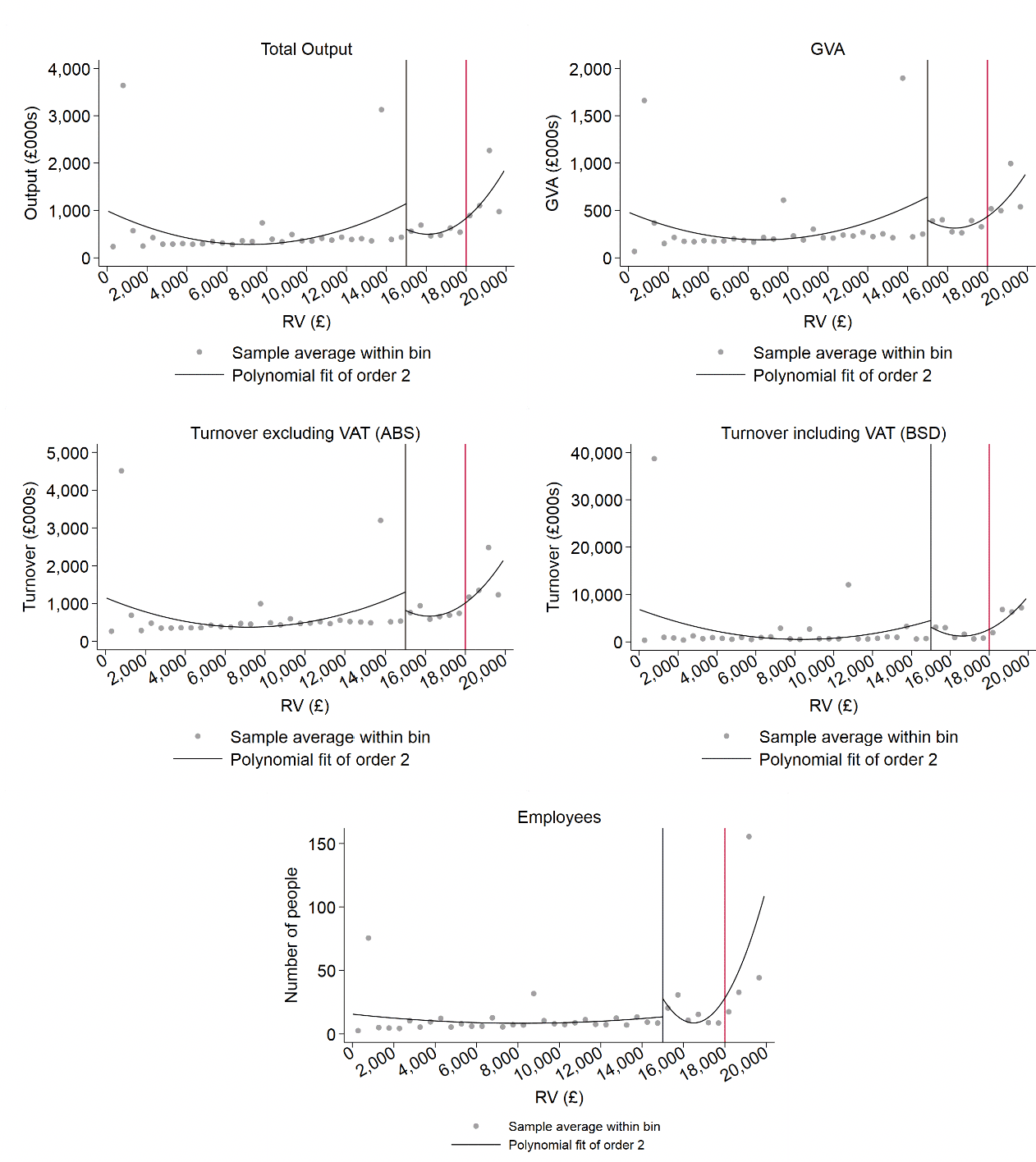
Note: Panels containing ABS turnover, total output and GVA are from the ABS and so use automatically use 3,749 fewer observations. Turnover including VAT (BSD) is in £000s. RV band widths are £500.
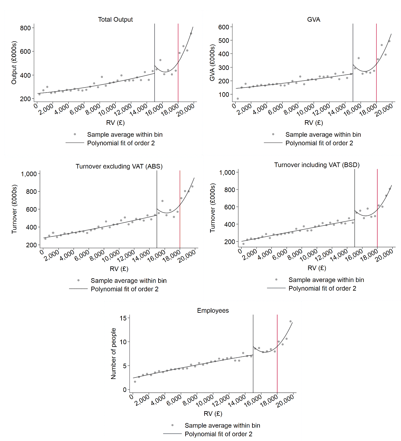
Note: Panels containing ABS turnover, total output and GVA are from the ABS and so use automatically use 3,749 fewer observations. Restrictions are turnover ABS, total output, GVA and turnover BSD <£5 million; employees < 100. This excludes 270, 100, 204, 664 and 360 enterprises respectively. Turnover including VAT (BSD) is in £000s. RV band widths are £500.
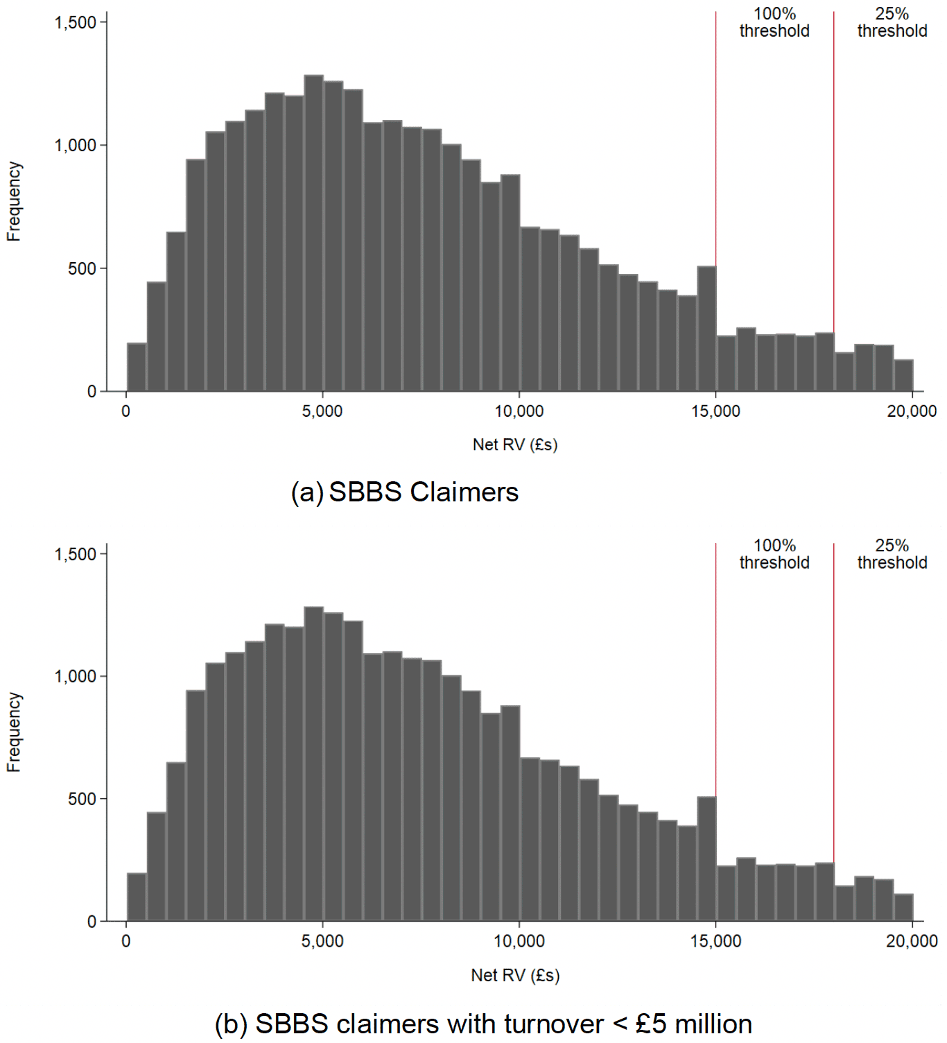
Note: Properties/enterprises are grouped into £500 RV bands. For example, the bar between 0-£500 groups all properties with an RV in the range.
7.7 Results
In Equation 6, we defined the regression discontinuity parameter as:
Throughout this section we have discussed the various ways in which the sample of properties included in the Scottish Government's matching exercise was slimmed down to a final sample with which this analysis would be carried out. We restrict the sample in one further way before estimating the effect of SBBS relief. Unfortunately, there are very few enterprises with an RV between £18,000 and £20,000. The variability in their outcomes is also large – see for example Table 7.6 and Figures 7.7 and 7.8. We therefore focus on estimating the effect of receiving 100% vs 25% SBBS relief (i.e., at the £15,000 threshold) as opposed to receiving 25% relief compared to zero (i.e., at the £18,000 threshold).
Given that turnover among enterprises just below the 25% threshold is high (Table 7.6), the effect of this 25% saving is likely to be proportionally far smaller relative to income for these businesses than for those just below the 100% threshold. Coupled with the small sample sizes available in practice, and increased variability in outcomes for businesses above the 25% threshold, it is unlikely that extending the analysis to compare the two groups would yield informative results.
As a result of this and the various other sample restrictions we have outlined to this point, the version of we might hope to estimate here can be best described as representing:
the expected change in outcome, on average, for the marginal single-site, single-property enterprise which is included in the IDBR if it received 100% as opposed to 25% SBBS relief.
However, as we have highlighted throughout the preceding sections, we are unable to estimate this net of any bias caused by the substantial bunching of enterprises around the 100% threshold. What we eventually estimate is more akin to the difference, on average, in recipients of 100% versus 25% SBBS relief at the margin. We proceed in estimating these parameters in order to understand at a high level whether or not any such differences exist.
To estimate this version of we must specify a functional form for the conditional expectation function . We allow for the following flexible function form:
Where is a non-parametric local polynomial function of RV, and is an error term. In estimating the effect of the policy, we specify two main versions of the above equation in which is linear and quadratic in RV respectively. We also weight observations closer to the threshold to a greater degree in calculating the expectations. This allows us to try and avoid a well-known source of bias in regression discontinuity estimates that arises from mis-specifying the functional form of . Lastly, and for a similar reason, we specify a bandwidth of £500 either side of the threshold within which we estimate the conditional expectation functions. That is, we primarily use the sample of enterprises for which their RV is between £14,500 and £15,500.
Table 7 below shows estimates of under the two specifications of described above. The panels respectively show estimates with outcomes () equal to:
- BSD turnover in thousands of pounds;
- BSD employment/number of employees;
- ABS turnover in pounds;
- ABS total output in pounds; and
- ABS GVA in pounds.
These are the main characteristics on which we have information in the BSD and ABS data we were provided. We note here that the ABS data is available for fewer enterprises, and so the estimates of effects on these outcomes automatically utilise fewer enterprises than those using the BSD. For the reasons outlined in the previous section, we do not use proxies of productivity as outcomes. Sample sizes are noted at the bottom of each panel in Table 7.7.
We use two samples: the "full claimer sample" (columns 1 and 3), which includes all single-site, single-property enterprises recorded as claiming SBBS relief; and samples that further impose, in each respective panel, that BSD turnover and ABS turnover, output and GVA are at most £5 million and BSD employment is less than 100 (these are identical to the restrictions in Figure 7.9 above).
Each cell of Table 7.7 represents the specification used to estimate the parameters. For example, column 2 in the first panel shows estimates of for turnover in the BSD using a linear and imposing the restriction that an enterprise's turnover be at most £5 million.
If receiving 100% SBBS relief compared to 25% has a beneficial effect on business outcomes, we expect the coefficient to be negative and statistically significant. This would indicate that business outcomes were worse in those businesses only receiving 25% SBBS relief compared to those receiving 100% SBBS relief.
However, the coefficient estimates in Table 7.7 are either all statistically insignificantly different from zero, or are significant and positive. This means we cannot conclude that receiving a higher level of relief is beneficial to businesses with RVs around the £15,000 threshold.
We noted earlier that we were concerned about the possibility that businesses had in some way 'endogenously' sorted into the RV band just below the threshold, and that were this the case, the estimates from our econometric analysis would be biased. Specifically, if those businesses with a higher need for support end up below the threshold, and these businesses have weaker business outcomes on average, then estimates of the effect of SBBS relief will be biased upwards. This is what we seem to find. Thus, we conclude that we cannot identify a local average treatment effect of the SBBS, noting that this is not a fault with the method but rather is a direct result of the bunching evident in the data.
One route through which businesses can influence which side of the SBBS threshold that they find themselves, is through the appeals process. In Appendix Table E.8 we attempt to understand how this might affect the results by including only those businesses that did not successfully appeal their 2016/17 valuation (we determine this by restricting the sample to those for whom both draft and final RV were identical). While this method is imperfect and may well raise its own issues (for example, a business might not have appealed due to a lack of perceived need for SBBS relief), the results are broadly similar for those in Table 7.7.
Moreover, it should be noted that none of the effects in either table are estimated with great precision, and in many cases the standard errors are more than a factor of ten larger than the estimated effects. This is due to the extreme degree of variability in the outcomes both across the threshold and within the RV groups; something we noted in Section 4 of this report. This variation still exists when restricting the sample in columns 2 and 4 of Table 7.7.
Second, the results in Table 7.7 are sensitive to the specification of particularly among the full sample. For example, comparing columns 1 and 3, the effect on turnover reduces by a factor of one-hundred to zero when accounting for a potential non-linearity in the conditional mean. The fact this effect is much less pronounced among the restricted sample again suggests variability among businesses in the same RV band is affecting the estimates.
| yi/yRD | Local linear | Local quadratic | ||
|---|---|---|---|---|
| (1) Full claimer sample | (2) Restrictions | (3) Full claimer sample | (4) Restrictions | |
| BSD Turnover (£000s) | 382.75* (212.55) | 115.82*** (40.64) | 3.96 (382.82) | 165.31*** (41.88) |
| N | 25,252 | 24,921 | 25,252 | 24,921 |
| Effective N | 1,241 | 1,215 | 1,241 | 1,215 |
| BSD Employment | 1.79 (1.96) | 1.32* (0.38) | 4.64 (3.80) | 0.71*** (0.14) |
| N | 25,252 | 25,097 | 25,252 | 25,097 |
| Effective N | 1,241 | 1,230 | 1,241 | 1,230 |
| ABS turnover (£000s) | 257.29* (55.23) | -9.93 (32.99) | 338.64* (46.55) | 35.88 (41.75) |
| N | 22,147 | 22,035 | 22,147 | 22,035 |
| Effective N | 1,093 | 1,081 | 1,093 | 1,081 |
| ABS output (£000s) | 128.24*** (36.73) | -33.85 (34.82) | 143.36* (79.07) | -39.81 (74.23) |
| N | 22,147 | 22,069 | 22,147 | 22,069 |
| Effective N | 1,093 | 1,085 | 1,093 | 1,085 |
| ABS GVA (£000s) | 154.92*** (30.92) | 16.94 (13.76) | 176.81*** (40.08) | 14.25 (38.56) |
| N | 22,147 | 22,117 | 22,147 | 22,117 |
| Effective N | 1,093 | 1,091 | 1,093 | 1,091 |
Note: *, **, and *** indicate statistical significance at 10%, 5%, and 1% respectively. Standard errors are in parentheses. Effective N is the number of observations within £1,000 of the 100% SBBS threshold. Panels containing ABS turnover, total output and GVA automatically use 3,749 fewer observations. Restrictions are turnover ABS, total output, GVA and turnover BSD <£5 million; employees < 100. This excludes an additional 270, 100, 204, 664 and 360 enterprises respectively.
Overall, Table 7.7 (or Appendix Table E.8) provides no evidence that there are differences in outcomes for the marginal recipients of 100% SBBS relief. It is important to make clear, however, that this should be interpreted as being that there is no evidence of an effect rather than there being evidence of the SBBS having no effect. The variability within RV bands, and the bunching around the SBBS threshold all undoubtedly contribute to our inability to identify any such differences.
Unfortunately, we cannot describe or quantify how or to what extent each or any of these factors plays a role. However, the large variability of business outcomes within RV bands even when SBBS relief is accounted for, which is much higher than variability between RV bands, underlines that RV is a very imprecise indicator of business need for support.
Throughout this portion of the analysis, we have broken down the overall estimation sample into three sub-samples of shops, offices, and industrial subjects in an attempt to understand whether: (1) this increases the likelihood we compare similar businesses; and (2) the effect of the SBBS differs across business types. Appendix tables E.5, E.6, and E.7 show our estimates of in each of these subsamples. Study of the coefficient estimates for these sub-samples reveals broadly the same conclusions as for the full sample.
Evidence of the SBBS having a positive effect on business outcomes would come from observing statistically significant negative coefficients in these tables: while there are a small number of significant negative coefficients, for example for ABS output and GVA for offices and industrial subjects, suggesting lower outcomes among those receiving 25% as opposed to 100%, the results are extremely sensitive to the specification (linear or quadratic) we use. As such (and in particular because of the issues of the high degree of variability in outcomes and bunching) we find no compelling evidence to reverse the conclusions drawn from the analysis of Table 7.7.
7.8 What can we infer from our econometric analysis?
Despite identifying a rigorous methodology with which we should be able to estimate the effects of the SBBS, we encountered a number of challenges that prevent us from implementing a fully robust evaluation. The over-arching conclusion from our econometric analysis is that we find no evidence that the SBBS, on average, is effective in promoting business outcomes for single-site, single-property businesses around the 100% SBBS threshold. This is true whether we analyse all businesses in our sample collectively, or disaggregate by type.
This is also true when we exclude those who successfully appealed their 2016/17 revaluation – a substantial source of bunching around the 100% SBBS threshold. This could be because there is actually no effect, but it could also be the case that: (1) the high level of variability in businesses with similar RVs and property types means we cannot adequately compare like-for-like; or (2) the endogenous bunching of businesses to the left of the 100% threshold is biasing an effect we would otherwise observe. Without an improved understanding of both, alongside improved data quality in this area to enable a full linking of businesses to properties, it is not possible to arrive at more definitive conclusions.
Nevertheless, the process of undertaking this analysis has highlighted some important facts that need to be recognised – in this case about the relationship between business outcomes and property RV. We documented that there is considerable variation in business outcomes for businesses with similar RV; indeed, there is much more variation in outcomes within RV bands than there is between RV bands. This brings into question whether RV – which is the primary basis on which SBBS eligibility is determined – is a good proxy for the need for business support.
We have, in addition, documented the difficulties we faced when matching the datasets. These difficulties are significant, and as a result the analysis presented here is based on a restricted data sample that may not be representative of the population of businesses as a whole. There are also challenges in identifying businesses in the data.
Contact
Email: ndr@gov.scot