Scottish Fire and Rescue Service (SFRS) - wildfire: incident reporting system - data analyses
This report examines Incident Reporting System (IRS) data on wildland fire incidents and uses these to improve the understanding of how upland wildfires start, investigate if wildfire occurrence differs between geographical areas; and describe how wildfires exhibit seasonal and temporal trends.
8 Relating wildfires to explanatory variables
8.1 Exploring wildfire-variables relationships
In this Section we explored relating the spatial distribution of selected IRS wildfires to information derived from readily available spatial layers of explanatory variables of fire, with the aim to improve our understanding of causative factors of wildfire ignition. We selected the Highland Local Authority (LA) to pilot this approach because previous analysis showed that this is where most bigger wildfires affecting important seminatural habitats (peatlands and heathlands) are more likely to occur.
We selected variables that are directly related to wildfire ignition and fire behaviour, shown in Table 8.1. These included:
- Bioclimatic variables (e.g., mean annual temperature and precipitation);
- Topography (elevation and slope);
- Variables related to accessibility and population densities (e.g., distances to nearest roads, settlements, and water features, along with the Urban Rural classification);
- Fuel type information at Broad Habitat (BH) level classified from the Land Cover Scotland 1988 (LCS88) map; and
- Two (2) integrated indices of socioeconomical factors (including employment, health, education, crime, and housing): the Rural Socio-economic performance index (SEP, Copus and Hopkins, 2015), which is a multivariate index devised to improve understanding of contemporary geographical variation in socio-economic characteristics in rural areas; and the Scottish Index of Multiple Deprivation (SIMD) 2020, which is the Scottish Government's official tool for identifying concentrations of deprivation in Scotland. Both datasets are available as maps at a Data Zone level. We used the actual numeric SEP index values for each Data Zone and the quantiles of SIMD that provide a measure of relative deprivation at Data Zone level.
| Code | Description | Type | Source | Processing | Reference |
|---|---|---|---|---|---|
| Bio1 | Annual mean temperature (oC) | Continuous | WorldClim v.2 (1970-2000) 1km grid resolution | Downscaled to 250m (bilinear transformation) | Fick and Hijmans (2017) |
| Bio4 | Temperature Seasonality (standard deviation ×100) | Continuous | |||
| Bio12 | Annual precipitation (mm) | Continuous | |||
| Bio15 | Precipitation Seasonality (Coefficient of Variation) | Continuous | |||
| Elev | Elevation above sea level in metres | Continuous | Ordnance Survey digital elevation model at 50m grid resolution (OS DTM 50) | Reclassified (by mean) to 250m grid resolution | OS Open Data |
| Slope | Slope (degrees) | Continuous | Derived from DTM 100m grid resolution | Zevenbergen and Thorne (1987) | |
| DistRoad | Distance to nearest road | Continuous | OS Open Roads network | Calculated using the Distance to nearest hub tool in QGIS 3.12 | OS Open Data |
| DistSettl | Distance to nearest settlement | Continuous | NRS Settlement boundaries (2016) | Open Government Licence (OGL) | |
| DistWater | Distance to nearest water feature | Continuous | OS Open Rivers | OS Open Data | |
| LCS88 | Land Cover of Scotland 1988 | Categorical | Macaulay Land Use Research Institute (MLURI, now The James Hutton Institute) | Broad Habitats (BH) based on Table 4.3. Grassland was separated as seminatural grassland and improved grassland | MLURI (1993) |
| SEP | Rural Socio -economic performance index | Continuous | https://www.hutton.ac.uk/ sites/default/ files/files/SEPDATA_RST.csv | Various national statistics linked to Data Zones 2001 | Copus and Hopkins (2015) |
| SIMD | Scottish Index of Multiple Deprivation (SIMD) 2020 | Categorical | https://spatialdata.gov.scot | SMDI Quantiles | OGL |
| UR8Fold | Scottish Government Urban Rural Classification (2016) | Categorical | https://spatialdata.gov.scot | Urban Rural 8- Fold classification | OGL |
We converted all datasets in Table 8.1 to raster layers with a specified spatial resolution of 250m grid cells. The spatial resolution was informed by the median nearest distance between recorded IRS wildfire location and the perimeter of burnt area polygons within the Highland LA (Table 6.1) and accounted for the known uncertainty in IRS fire incident locations. We extracted the values of the variables in Table 8.1 at the locations of the wildfire incidents that fell within the Highland LA, which resulted to a dataset of complete values for all variables for 1,752 of the 1,852 Highland LA wildfires.
Table 8.2 gives the descriptive statistics for the continuous (i.e., numeric) explanatory variables at wildfire locations. Based on median values, wildfires in the Highland LA tend to occur in warmer and drier areas of relatively low altitude and relief that are to a certain extent close to the road network. Based on the Urban Rural classification, 61% of Highland wildfires occurred in very remote rural areas, followed by 22% that occurred in remote rural areas. Around 32% of Highland wildfires were on shrub followed by fires on improved grassland (16%), conifer forest fires (15%), seminatural grassland fires (14%) and peatland fires (11%). Most wildfires fell into the 3rd and 4th SIMD quantiles (36% and 22%, respectively), while the median SEP index was at 6.1.
| Covariates | Min | Median | Mean | Max |
|---|---|---|---|---|
| Bio1 | 4.9 | 8.1 | 8.1 | 9.8 |
| Bio4 | 295.7 | 385.4 | 383.7 | 442.8 |
| Bio12 | 644.2 | 1,722.9 | 1,603.6 | 2,643.6 |
| Bio15 | 17.0 | 32.5 | 30.2 | 39.2 |
| Elev | 0.7 | 61.8 | 96.9 | 711.3 |
| Slope | 0.1 | 4.4 | 5.7 | 30.0 |
| DistRoad | 126.0 | 408.0 | 499.6 | 3,837.0 |
| DistSettl | 2.0 | 136.5 | 206.6 | 1,840.0 |
| DistWater | 1.0 | 154.0 | 210.0 | 2,017.0 |
| SEP | 0.0 | 6.1 | 5.9 | 8.3 |
8.2 Ignition risk mapping
Building the dataset of spatial relationships between wildfires and explanatory variables enabled us to explore modelling and mapping ignition risk in the Highland LA using statistical methods. The objective of this analysis was to demonstrate how the IRS wildfires can be utilised to produce ignition risk maps that can be used alongside other datasets, e.g., maps of fire danger predictions, to assist in wildfire preparedness and prevention and mitigation planning.
Several recent studies have utilised a logistic regression approach to mapping wildfire ignition risk (e.g., Catry et al., 2009; Dixon and Chandler, 2019), while ensemble decision trees, such as the Random Forests (RF) algorithm (Breiman et al., 1984), are also robust alternative methods to logistic regression for modelling non-linear relationships (Kirasich et al., 2018). Both approaches of predictive modelling treat the wildfire incidents as the dependent variable, while the information extracted from the explanatory variables at wildfire locations are used as the model predictors. The result of this modelling exercise is a map of probabilities of ignition (0-1) that can be classified into risk classes to produce an ignition risk class map or to produce a map of wildfires based on specified thresholds of probability ignition. An additional important output of the modelling are metrics of relative importance of the different explanatory variables used as predictors of fire ignition risk, which can provide some causative explanation of wildfire occurrence in the study area.
The models require non-ignition sample points as well as the ignition points (i.e., wildfire locations) for training. Following the approach by Dixon & Chandler (2019), we randomly selected non-ignition points within the study area, excluding areas within 250m of a known ignition to ensure that no ignition point was accidently included as a non-ignition point. Around twice as many non-ignition (3,682) than ignition (1,752) points were created, to better represent the greater spatial coverage of non-ignitions compared to recorded wildfires. As in the case of the ignition points/wildfires, we also extracted variable/predictor values at the locations of non-ignitions and merged them with the wildfires and variable values dataset. We used a 70% random sample of the merged dataset for training the model (3,805 points), leaving 30% for independent testing/validation (1,629 points not used for training the models). After building the ignition risk model, it was spatially deployed using the predictor maps to produce maps of probabilities of ignition risk at a 250m grid resolution for the Highland LA.
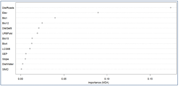
We built ignition risk models using both logistic regression and RF. Here, we present the results from the RF modelling because RF performed better than logistic regression in this case. We were also keen to explore RF because we have substantial experience in using it (e.g., Gagkas and Lilly, 2009) for environmental modelling and because RF are a machine-learning algorithm with many advantages for complex modelling, such interpretability, their ability to deal with missing data and with autocorrelated variables and their ability to utilise both discrete (i.e., categorical) and numeric predictors (Liaw and Wiener, 2002). Ignition risk was predicted with RF using binary classification (ignition vs non-ignition) and with fine-tuning algorithm parameters such as the number of classification trees generated. Variable importance was calculated using the mean decrease accuracy (MDA), which gives the average accuracy for the predictor minus the decrease in accuracy after permutation of the predictor.
Overall, RF models produced had very high accuracies of above 90%; this was expected to a certain degree because there are relatively clear, end hence relatively easy to model, patterns of wildfire occurrence in the Highland LA. We would expect smaller accuracies if building an ignition risk model covering the whole of Scotland that had to model more complex patterns and interactions between wildfire occurrence and variable spatial variation. Distance to the nearest road was the most important model predictor (Figure 8.1), which is consistent with findings from similar studies, e.g., as in the Peak District National Park (Dixon and Chandler, 2019), followed by elevation and bioclimatic variables (annual temperature and precipitation). The importance of accessibility and proximity to populated areas was also highlighted by the fact that both distance to settlements and the Urban Rural classification scored relatively high in terms of MDA. Fuel type (based on LCS88) and the socioeconomical indices gave low MDA scores; this is explained by the relatively moderate variability in fuel type composition and predominant remote rural character of the Highland LA that exhibited little spatial variation of SIMD and SEP values. It is expected that the relative importance of fuel types and socioeconomic indices would be greater when developing a national cover ignition risk model due to the greater spatial variation of these variables at national scale and the presence of more complex interactions than those in the Highland LA.
Results of independent testing using the left-out sampling points (Table 8.3) showed very high sensitivity (0.97), i.e., the avoidance of false negatives (predicting non-ignition where actually there was an ignition). The model's specificity was also high (0.87), highlighting its good ability to avoid predicting false positives (predicting ignition where actually the cell was non-ignition). We used a 0.6 threshold (i.e., the model predicts "fire" if there is a >60% probability of a fire occurring at this location) to calculate these statistics. As Dixon and Chandler (2019) note, the user should make this threshold decision, as the cost of a false positive is likely not equal to the cost of a false negative. For example, attending a call-out in which no ignition has occurred may be preferable to not attending a call-out in which there is an ignition. Therefore, it might be preferable to set higher thresholds to reduce the likelihood of a false negative (the model predicts no ignition when actually there is an ignition).
| Predicted non-ignition | Predicted ignition | |
|---|---|---|
| Actual non-ignition | 1,074 (True negative) | 59 (False positive) |
| Actual ignition | 28 (False negative) | 466 (True positive) |
Figure 8.2 shows the locations of predicted locations of wildfires using a probability threshold of 0.6, and Figure 8.3 shows predicted wildfire locations in relation to burnt area polygons in two identified hotspots of predicted fire occurrence.
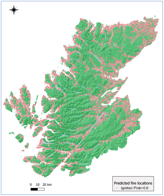
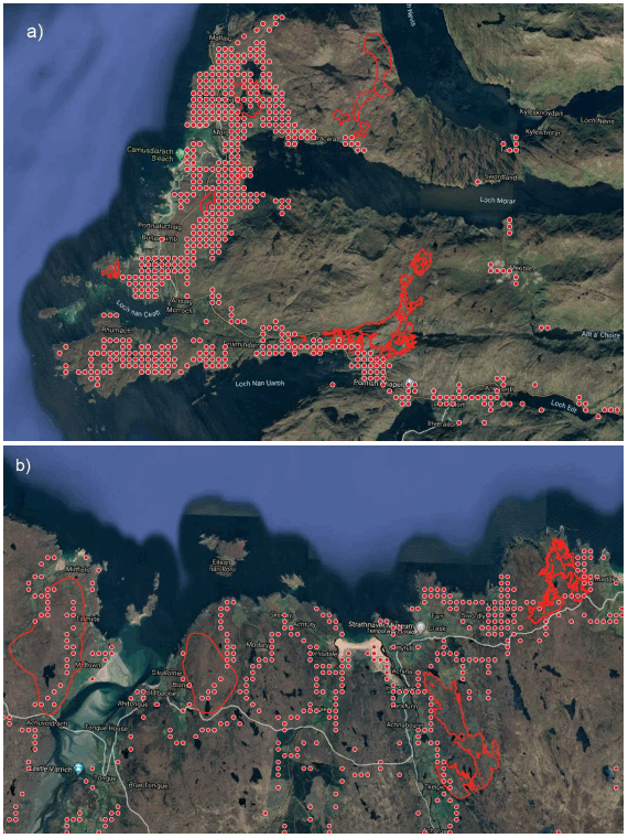
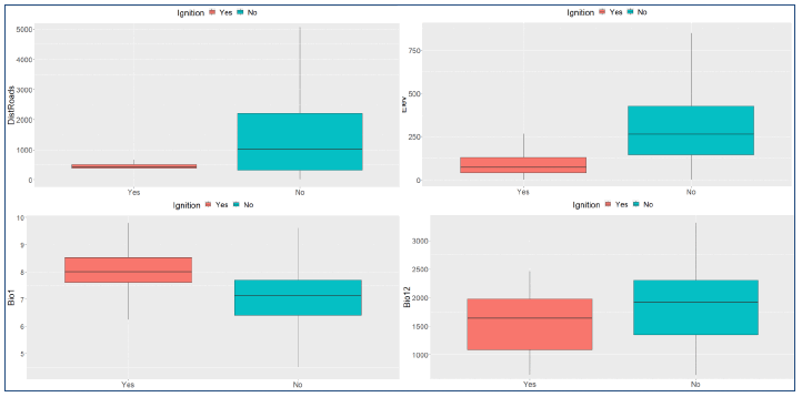
Overall, the ignition risk model succeeded in predicting fire locations in close proximity to almost all available burnt area polygons, most often close to the existing road network. We need to stress that the results of this modelling show the locations where a successful ignition is likely to occur and not the areas where the fire is likely to spread. The range of values of selected variables for predicted fire locations (ignition probability >0.6) and non-ignitions (ignition probability <0.6) (Figure 8.4) shows clear distinctions in variable values, such as distance to roads and annual precipitation, between ignition and non-ignition locations. In addition, a slightly greater proportion of predicted ignitions was in accessible rural areas (7%) compared to non-ignitions (4%), while 77% of predicted ignitions was in very remote rural areas compared to 83% of non-ignitions. Regarding fuel types, the model predicted a greater proportion of fires in seminatural grasslands and conifers (both 14%) compared to non-ignitions (8% and 5%, respectively), whereas more non-ignitions (in proportion) were predicted in shrublands and peatlands (46% and 21%, respectively) than ignitions (16% and 38%).
Overall, the results of the Highland LA case study show that models built using a statistical approach can provide objective assessments of the relative importance of explanatory variables of fire occurrence. In addition, predictive models can provide accurate spatial predictions of ignition risk and hence can become a useful tool for wildfire preparedness and mitigation planning. However, we need to stress that these purely data-driven approaches require extensive "sense checking", ensuring that the variables selected make physical sense and that the identified patterns and relationships are sound conceptually and are not simply statistical artefacts.
Contact
Email: alison.seton@gov.scot