Improving Our Understanding of Seabird Behaviour at Sea

3 Results

3.1 Northern Gannet

3.1.1 Comparison of wind speed use vs availability

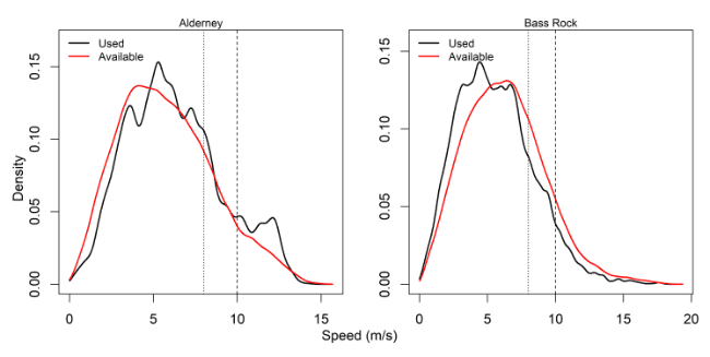
Comparisons of wind speeds experienced and those available within the wider area were made for all colonies – see Table 3, Figure 2 and Appendix AB.

For Bass Rock, values of proportional use were slightly lower than available for Bass Rock for both 8 m/s and 10 m/s splits of the dataset, whereas at Alderney the reverse was true. It is not possible here to fully tease out these drivers, which would require further analysis, however, these differences may reflect colony variations in foraging activity.

Table 3: For Gannet, summary of the proportions of tracking data by wind speed thresholds of more than 10 m/s or more than 8 m/s, and further comparing wind speeds encountered by birds ('used') vs wind speeds 'available'. Assessment is made both (i) within the full months that tracking was carried out and (ii) for the precise tracking date-times, for all Copernicus grid squares that birds overlapped with; proportions for 'use' data are calculated on the data modelled within HMMs, thus each data point is a GPS fix; for 'available' calculations, each data point is an hourly wind speed estimate for each Copernicus grid square.

		Used (%)		Available (tracking period, %)		Available (all months, %)
Colony / State	Tracking months and years	8 m/s	10 m/s	8 m/s	10 m/s	8 m/s	10 m/s
Alderney	Jun 2011, 2013 – 2015	25.61	12.22	21.33	8.41	23.22	8.74
Bass Rock	Jul – Aug 2010, Jun – Aug 2011, Jul – Aug 2012, Jun – Aug 2015	19.01	6.53	26.42	10.4	28.56	12.04

3.1.2 Model summary

For Alderney and Bass Rock mean step lengths (from gamma distribution) and angle parameters (mean and concentration from Von Mises) for each state are shown in Table 4 below. These indicated consistent direction for slower floating on the sea State 1 and faster commuting State 2, in contrast to State 3 with wider turning angles and a lower consistency in direction between fixes (Appendix AC).

Table 4: For Gannet, summary of mean ± SD step length and turning angles (mean, concentration) for each site.

	Step			Turn
Colony / State	1 (floating)	2 (commuting)	3 (forage/ search)	1 (floating)	2 (commuting)	3 (forage/ search)
Alderney	96.35 ± 52.24	1645.48 ± 440.29	322.18 ± 397.34	0, 61.51	0, 18.98	0, 0.95
Bass Rock 2010	42.31 ± 22.36	1772.07 ± 410.64	360.39 ± 470.03	0, 14.38	0, 22.92	0, 0.55
Bass Rock 2011	46.53 ± 24.74	1636.53 ± 385.42	333.88 ± 431.06	0, 16.18	0, 19.11	0, 0.47
Bass Rock 2012	42.75 ± 21.63	1761.88 ± 435.62	409.61 ± 499.06	0, 13.22	0, 21.07	0, 0.49
Bass Rock 2015	35.85 ± 18.49	1737.19 ± 410.03	423.63 ± 535.22	0, 26.94	0, 49.08	0, 1.35

For Bass Rock, models were run separately for each year (see methods and Appendix AC). Mean step lengths and turning angles, however, were fairly consistent across the four year-specific models (2010 – 2012, 2015), hence we do not believe that this meaningfully changed the behavioural classifications between years for this colony as a result of using slightly different step and turning angle distributions per year for specifying behavioural classifications.

At all colonies, direct transitions to and from states 1 (floating) and 2 (commuting) were rarer in the datasets (see Dean et al. 2013). Most frequently, fixes following a particular state were most likely to be classified as the same state again. However, where switches did occur, typically floating on the sea was preceded and succeeded by locations classified as state 3, with further switches occurring between commuting and foraging (Appendix AC).

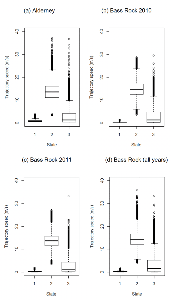
3.1.3 Travel speeds

Models indicated that during commuting (using the mean parameter estimate above), on average (over other covariates), Gannets flew at a mean of 13.60 m/s and 14.37 m/s for Alderney and Bass Rock (Table 5, see also Figure 3); note for Bass Rock models from individual years were used, which are broken down further in Table 5. Note, these values were obtained across headwinds and tailwinds, and given slower travel in stronger headwinds, and faster travel in tailwinds (Appendix AD), represent the mean wind travel speed at mean wind speed with no directional bias during commuting. Foraging/searching speeds were low, and often lower than that speed expected to be needed to sustain powered flight, suggesting strongly much of the activity for State 3 included other behaviours associated with foraging, such as diving, and associated phases on the sea (see Section 2.3.9 for further anticipation of this bias).

Table 5: For Gannet, summary of speeds per state (m/s), as obtained through classification of tracking data using HMMs.

Colony / State	1 (floating)	2 (commuting)	3 (forage/search)
Alderney	0.72 (0.47 – 1.05)	13.60 (11.15 – 16.01)	1.25 (0.34 – 4.15)
Bass Rock 2010	0.32 (0.21 – 0.45)	14.78 (12.53 – 17.00)	1.28 (0.28 – 4.87)
Bass Rock 2011	0.35 (0.28 – 0.51)	13.70 (11.55 – 15.72)	1.27 (0.30 – 4.38)
Bass Rock 2012	0.35 (0.22 – 0.46)	14.53 (12.18 – 16.96)	1.77 (0.42 – 5.53)
Bass Rock 2015	0.27 (0.18 – 0.39)	14.33 (12.25 – 16.54)	2.15 (0.40 – 5.88)
Bass Rock (all yr)	0.31 (0.21 – 0.45)	14.37 (12.16 – 16.63)	1.58 (0.35 – 5.24)

3.1.4 Effects of wind speed on step length (speed)

For Alderney, models specifying a simple effect of wind speed on step length showed a general (shallow) decreasing trend in step length over increasing wind speed for commuting (β = -0.056), corresponding to a ca. 500 m (per 2 min) reduction in step length (ca 4.2 m/s travel speed) over increasing wind speed (between 0.03 – 14.0 m/s, corresponding to standardised wind speeds (-2.21 – 3.02) (Appendix AE). Slight increases in step lengths were recorded for floating on the sea and foraging (β = 0.016, β = 0.006). Similarly, for Bass Rock (Appendix AE), individual year models also showed negative beta coefficients for wind speed and commuting (2010, β = -0.040; 2011, -0.053, 2012 -0.054, 2015 -0.033), and (mainly) increases for floating (β = 0.046, β = -0.010, β = 0.018, β = 0.032) and foraging (β = 0.020, β = 0.038, β = 0.054, β = 0.031). For commuting, such patterns with wind speed alone (without any directional component), are likely due to the negative effects of crosswinds and headwinds, outweighing the positive gains from headwinds, but also linked to complexities of colony location and route taken on outward and inward commutes during trips, and the prevailing wind speed and direction over the tracking period; for instance during 2011, winds were more northerly and north-westerly than westerly mean flows in 2010, which could have affected relationships compared to other years; however, patterns with head and tail winds reveal much clearer patterns with commuting (Appendix AE).

For Alderney, models for Gannets including effects of wind speed*angle_osc, showed a strong positive coefficient value for the interaction (wind speed:angle_osc β = 0.408), indicating faster commuting speeds in faster tailwinds (angular_osc -1 = headwind, +1 = tailwind), and the opposite in a headwind. There was little influence of birds aligning commuting with prevailing wind directions, i.e. turning with the wind during commuting (β = -0.012). Similarly, for Bass Rock, wind speed:angle_osc parameters were as follows: β = 0.407, 0.431, 0.387 and 0.358 for 2010 – 2012 and 2015, respectively, indicating the same general pattern (Appendix AE).

3.1.5 Transition effects between states in relation to covariates

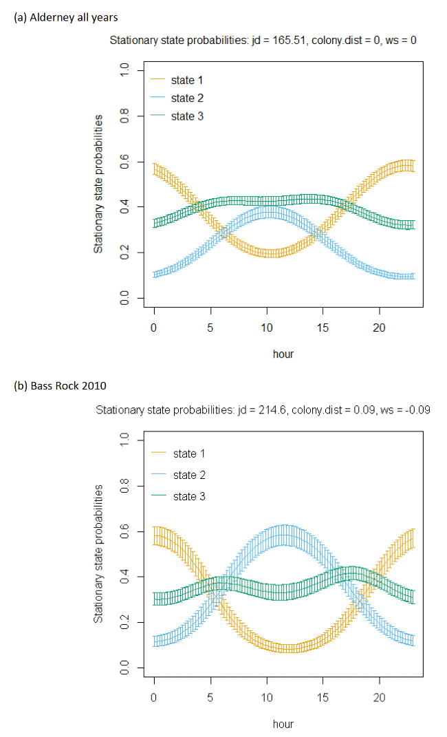
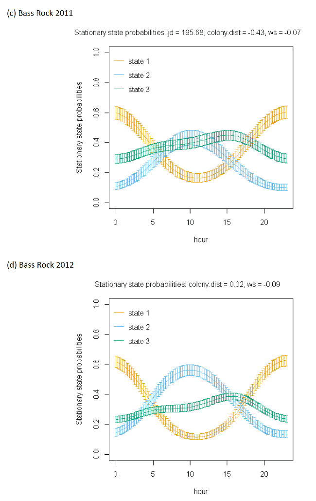
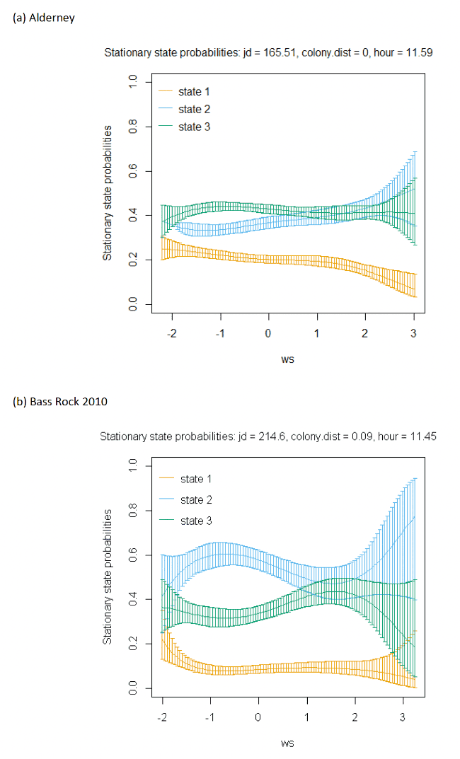
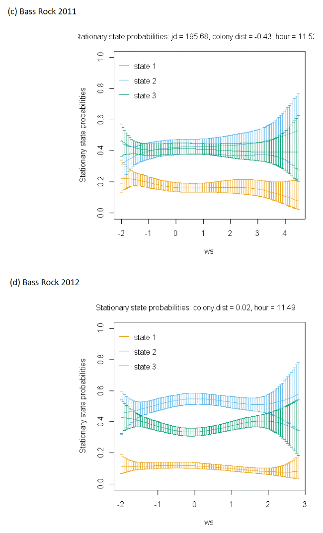
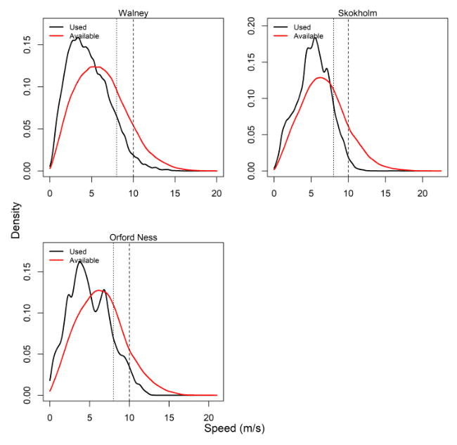
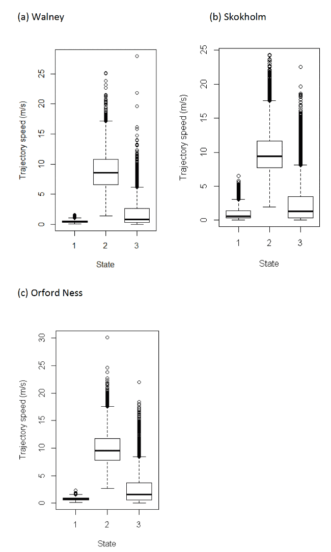
The best-fitting model, as assessed by AIC, was the full model with all covariates, being best across all colonies (Appendix AF); transition and stationary state probability plots are given in Figure 4, Figure 5 and Appendix AD.

As with other species, there were clear patterns for each of the three colonies in distance from the colony at which transitions occurred from floating to commuting and commuting to foraging (see Appendix AG). Over Julian date patterns across the gannet datasets were varied and less clear given the shorter time span for this variable included in models (as compared to Lesser Black-backed Gulls where a wider period of time could be modelled).

As with other species, the models showed very strong patterns over hour of the day. At both colonies, gannets were much more likely to be floating on the sea overnight and foraging and commuting in the day. For Bass Rock, patterns across years were also similar, and matched those of Alderney, with a small double peak in stationary state classifications seen for foraging/searching across the day, and similar timing of a peak in commuting behaviour, at the expense of reduced probability of remaining in State 1 (floating on the sea) between times t and t + 1.

Spline models for the wind speed variable indicated a complex pattern over increasing wind speed. Typically, the probability of a bird remaining in the state of floating decreased as wind speed increased, switching to foraging/searching, although for Bass Rock 2012 the spline was less strong. These patterns were clearer when investigated further as a simplified linear term in interaction with the variable angle_osc for alignment of travel with wind direction.

In headwinds the probability of remaining in the floating State 1 between time t to t+1 decreased over increasing wind speed. However, the probability of switching from floating to foraging from time t to t+1 in a headwind increased over increasing wind speed. This pattern was evident but less apparent for Alderney. However, at both Bass Rock and Alderney, the balance of remaining and switching between different states yielded a similar stationary state probability for floating on the sea, with, particularly at Bass Rock very strong patterns in birds being classified as floating as head-wind speed increased.

When viewed in terms of the varying tail- and headwind spectrum of values (+1 to -1) at the strongest wind speeds where patterns were most pronounced, the patterns observed were similar for gannets compared to other species in this study. As winds veered towards a headwind (-1), clear increases in commuting time and reductions in floating time were seen in stationary state probabilities with foraging/searching increasing markedly with increasing. For tailwinds, birds remained in the state of floating (t to t + 1) more often, and did not switch as often to foraging/searching, which for Bass Rock in particular, further resulted in reduced time spent foraging/searching in tailwinds, although for Alderney the pattern indicated relatively consistent foraging over the head-tail wind spectrum.

3.1.6 Time in states

The range of duration of data per bird and the proportion of time spent in different states are shown in Table 6. As birds with fewer data had less time to demonstrate their overall time spent in different states, we used information from birds with more than ten hours of data, to exclude any very small tracking durations that could otherwise skew any patterns.

Table 6: For Gannet, estimated time spent in states for each colony for birds at each colony across years; note occasionally initial movement models could not be fitted due to a lack of data available for some individuals, hence the effective sample size feeding into assessments is provided in brackets.

			Duration of tracking			Proportion time spent per state
Colony	No. birds total (modelled)	Years	No. birds > 10 hrs tracking data	Duration (hrs) mean ± SD per bird	Tracking data range (hrs)	1 floating mean ± SD	2 commuting mean ± SD	3 foraging / searching mean ± SD
Alderney	61 (61)	2011, 2013 – 2015	58	107.36 ± 62.43	5.1 – 234.1	0.36 ± 0.09	0.27 ± 0.07	0.37 ± 0.08
Bass Rock	133 (133)	2010 –2012, 2015	130	101.13 ± 44.94	3.8 – 270.4	0.32 ± 0.08	0.35 ± 0.13	0.35 ± 0.10

3.1.7 Utilisation distributions

Figures depicting utilisation distributions for each colony are shown in Appendix AH – see also methods for further description. Depending on the colony, there was a smaller amount of data from the very highest wind speeds (greater than 8 m/s) – see also section above comparing use and availability for wind speed distributions.

Where sample sizes of number of fixes and birds used to compute utilisation distributions was low, here taken as less than 100 fixes and less than five birds for the lowest amounts of data (see Appendix AA and methods), then confidence in the overlap result is considered lowest, and is here indicated as requiring a high degree of caution in interpretation of results. Also highlighted is the proportion of fixes available per split of data, with proportions of less than 5% of the total for the state also flagged up as requiring caution.

For gannets, sample sizes are here considered sufficient for both Alderney and Bass Rock in different conditions based on these sample size criteria. However, we also caution the comparison between utilisation distributions with very different sample sizes, as this in itself a recognised issue (see methods). Further, night-high wind categories for both colonies for the state of commuting and the night-high foraging/searching category at Bass Rock represented less than 5% of the total data for each state per colony.

3.1.8 Overlap indices

Overlaps between states in different conditions and times of the day are visualized in Appendix AI, and summarised in Table 7.

For Alderney, most 95% KDEs, representing total area usage, showed moderate to very high levels of overlap (ca. 0.4+, see methods, one being a perfect match and zero being completely different) between the daytime low-wind conditions (taken here as representative of similar conditions that aerial surveys would encounter), and the other scenarios of day-high wind, night-low wind and night-high wind scenarios across different states; highest overlaps in distributions were seen for day-low vs day-high conditions for commuting (state 2, BA = 0.9) and least for day-low vs night-high for State 3 foraging (BA = 0.53). Core area use (represented by 50% KDEs) showed that there were lower overlaps that for 95%, being between 0.14 (very low overlap, day-low vs night-high foraging) and 0.73 (day-low vs day-high, for commuting). We also note that State 1 floating had consistently lower 95% and 50% KDE overlaps than other states.

For Bass Rock, similar to Alderney, State 1 resting showed lower overlaps for day-low vs other conditions, with the lowest overlap for total area use (95% KDE) for day-low and night-high (low degree of overlap, BA = 0.4), and equal lowest overlap of the core 50% KDE for the same pairwise comparison. Highest overlaps at Bass Rock for both the 95% and 50% KDEs were seen for the day-low vs day-high comparison of commuting (BA = 0.88, 'very high' overlap and 0.72, 'high').

For both colonies across states, overlaps for the night-high vs night-low comparison (min 95% KDE, BA = 0.44; min 50% KDE, BA = 0.17, Bass Rock floating state) were slightly lower than day-high vs day-low comparisons (min 95% KDE, BA = 0.52; min 50% KDE, BA = 0.19, Bass Rock floating state). However, for both colonies, there were bigger differences when comparing day-low and night-low, and day-high and night-high; BA indices were higher (for 95% and 50% KDEs) between day and night in low wind conditions, than comparing day and night in high wind conditions, which was true across all states (e.g. lowest 95% KDE BA indices across colonies and states for daytime low vs night low = 0.69 compared with day-high vs night-high, BA = 0.46, again for Bass Rock floating state). In generalising, this may indicate a stronger driver of wind speed than time of day for distributions.

Table 7: For Gannet, overlap indices (Bhattacharyya's Affinity Index) for pair-wise combinations of utilisation distribution assessing similarity in 95% KDEs (and 50%, brackets) for different levels of day and night, and high/low wind and States 1, 2 and 3 (floating, commuting and foraging/searching); bold highlights indicate comparisons of greatest interest, comparing the equivalent conditions when surveys are made (low wind daytime) to other conditions.

(a) Alderney

state		day.high	day.low	night.high
Floating (state 1)	day.low	0.61 (0.34)
	night.high	0.54 (0.25)	0.55 (0.21)
	night.low	0.53 (0.28)	0.75 (0.58)	0.53 (0.2)
Commuting (state 2)	day.low	0.9 (0.73)
	night.high	0.62 (0.29)	0.58 (0.26)
	night.low	0.65 (0.31)	0.74 (0.39)	0.51 (0.21)
Foraging/searching (state 3)	day.low	0.75 (0.6)
	night.high	0.54 (0.21)	0.5 (0.14)
	night.low	0.58 (0.39)	0.78 (0.68)	0.49 (0.15)

(b) Bass Rock

state		day.high	day.low	night.high
Floating (state 1)	day.low	0.52 (0.19)
	night.high	0.46 (0.22)	0.4 (0.15)
	night.low	0.44 (0.16)	0.69 (0.49)	0.44 (0.17)
Commuting (state 2)	day.low	0.88 (0.72)
	night.high	0.62 (0.4)	0.65 (0.38)
	night.low	0.79 (0.65)	0.87 (0.8)	0.62 (0.39)
Foraging/searching (state 3)	day.low	0.68 (0.33)
	night.high	0.51 (0.24)	0.46 (0.15)
	night.low	0.56 (0.25)	0.74 (0.53)	0.45 (0.16)

3.2 Lesser Black-backed Gull

3.2.1 Comparison of wind speed use vs availability

Comparisons of wind speeds experienced and those available within the wider area were made for all colonies – see Table 8, Figure 6 and Appendix AB.

For all Lesser Black-backed Gull colonies, the conditions that birds experienced revealed much lower percentages of use of wind speeds more than 8 m/s and 10 m/s, compared to that available over the tracking period and the full months in which tracking was carried out (Appendix AB). The tracking period availability also closely matched that available within the months of tracking, since the attachment method for gulls in this study was a harness, which lasted over long period, thus covering the majority of the months in which tracking was conducted.

The apparent lack of use of high winds was therefore pronounced for Lesser Black-backed Gulls. This is due to a couple of different reasons – the use of offshore areas for Lesser Black-backed Gulls is biased to particular times in the breeding season, typically the mid to -late chick rearing period ca. June-July (see e.g. Thaxter et al. 2015). At other times, area use is inshore and coastal and so has not been included in these assessments. Further, the data included for use-availability assessment includes a wide period of the year from March to August, when Lesser Black-backed Gulls were associated with their breeding colony. Given there is a lack of use of offshore areas at times of the year such as March and April (typically pre-breeding) when conditions are likely much windier offshore, and use of offshore areas in June – July being more likely to coincide with periods of calmer weather, this would explain the lack of use of high wind speeds for this species.

Table 8: For Lesser Black-backed Gull, summary of the proportions of tracking data by wind speed thresholds of more than 10 m/s and more than 8 m/s, and further comparing wind speeds encountered by birds ('used') vs wind speeds 'available'. Assessment is made both (i) within the full months that tracking was carried out and (ii) for the precise tracking date-times, for all Copernicus grid squares that birds overlapped with; proportions for 'use' data are calculated on the data modelled within HMMs, thus each data point is a GPS fix; for 'available' calculations, each data point is an hourly wind speed estimate for each Copernicus grid square.

		Used (%)		Available (tracking period, %)		Available (all months, %)
Colony / State	Tracking months and years	8 m/s	10 m/s	8 m/s	10 m/s	8 m/s	10 m/s
Walney	May – Aug 2014, Mar – Aug 2015 – 2018	10.68	2.83	26.04	11.2	26.76	11.33
Skokholm	May – Aug 2014, Mar – Aug 2015 –2017	11.96	1.77	31.69	14.27	31.98	14.67
Orford Ness	Jun – Aug 2010, Mar – Aug 2011 –2015	13.3	3.31	28.68	12.25	27.79	11.62

3.2.2 Model summary

Three-state offshore model

For each colony, mean step lengths (from gamma distribution) and angle parameters (mean and concentration from Von Mises) for each state are shown in Table 9 below. Together these models indicated more consistent direction for slower floating State 1 and faster commuting State 2, in contrast to State 3 with wider turning angles and a lower consistency in direction between fixes (Appendix AC).

Table 9: For Lesser Black-backed Gull, summary of mean ± SD step length and turning angles (mean, concentration) for each site.

	Step			Turn
Colony / State	1 (floating)	2 (commuting)	3 (forage/ search)	1 (floating)	2 (commuting)	3 (forage/ search)
Walney	143.10 ± 70.84	2647.87 ± 913.43	553.26 ± 681.72	0, 59.44	0, 6.02	0, 0.31
Skokholm	267.23 ± 212.73	2953.14 ± 931.75	704.21 ± 814.41	0, 42.21	0, 12.99	0, 0.72
Orford Ness	228.99 ± 92.09	2995.43 ± 896.05	786.32 ± 834.20	0, 169.93	0, 10.30	0, 0.78

At all colonies, direct transitions to and from States 1 (floating) and 2 (commuting) were typically rarer in the datasets, as also found in some other studies (see Dean et al. 2013). Most frequently, fixes following a particular state were most likely to be classified as the same state again. However, where switches did occur, floating on the sea was typically preceded and succeeded by locations classified as State 3, switches relatively frequently occurred between commuting and foraging, generally being most consistent for commuting and foraging.

Four-state offshore model

Four-state models indicated that a further stationary state could be identified from the datasets, that may represent birds perching at sea or on land away from the breeding colony, or other behaviours such as preening or social interactions on the sea surface when not in flight. Comparing this model to the three state model, generally involved differing classifications of the "foraging/searching" and "floating on sea" states from the original three state model; note, commuting was more consistently classified between three and four state models. For example, for Walney, a four-state model gave mean step lengths for each state as 135.03 ± 137.54, 149.96 ± 76.34, 2846.75 ± 869.89 and 1216.65 ± 841.87 for "stationary", "floating on the sea", "commuting" and "foraging/searching respectively" (States 1-4 for the four-state approach), with concentration parameters for the von Mises angle distribution given as 0.21, 70.10, 10.52 and 0.79 for each state respectively. Thus as with the three-state model, commuting and floating on the sea had more consistent direction, differing by speed distinctions, and similarly, slow potential perching behaviour had similar wide turning angles between fixes, t and t+1, differing in speed delineations.

3.2.3 Travel speeds

Three-state model

The Lesser Black-backed Gull models can be used to estimate travel speeds in each state. During commuting (using the mean parameter estimate above), on average (over other covariates), Lesser Black-backed Gulls travelled at a mean of 8.83 m/s, 9.84 m/s and 9.98 m/s for Walney, Skokholm and Orford Ness; these values were obtained across headwinds and tailwinds, and given slower travel in stronger headwinds, and faster travel in tailwinds (Appendix AE), represent the mean wind travel speed at zero wind speed with no directional bias during commuting.

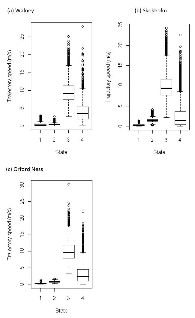
Table 10 below shows the distributions of speeds from boxplot analysis (Figure 7) after assigning states back to the raw data. As with other species in this study, we note, however, that precise behaviours within this broad category of foraging/searching could also include non-flight activities. Further, for gulls in particular, "foraging/searching" could also encompass perching activity if birds rest on structures at sea away from the colony – see methods Section 2.3.9. A further four-state model was specified for this species – see below.

Table 10: Lesser Black-backed Gull, summary of speeds per state (m/s), as obtained through classification of tracking data using three-state HMMs.

Colony / State	1 (floating)	2 (commuting)	3 (forage/search)
Walney	0.49 (0.27 – 0.79)	8.59 (6.61 – 10.83)	0.84 (0.29 – 2.65)
Skokholm	0.58 (0.33 – 1.43)	9.41 (7.71 – 11.64)	1.35 (0.37 – 3.46)
Orford Ness	0.77 (0.55 – 0.96)	9.54 (7.80 – 11.71)	1.62 (0.61 – 3.73)

Four-state model

Four-state HMMs estimated a further state of "perching", separate to the existing three states above, and generally involved differing classifications of the "foraging/searching" and "floating on sea" states from the three state model (Table 11); the state of commuting (here now given as State 3, from the four-state model) was more consistently classified between three- and four-state models. The perching state identified from the four-state model was identified at very slow speeds and thus the foraging/searching state was greater, and therefore was potentially representative of a greater proportion of in-flight activity compared to the three-state model.

Table 11: For Lesser Black-backed Gull, summary of speeds per state (m/s), as obtained through classification of tracking data using four-state HMMs.

Colony / State	1 (perching)	2 (floating)	3 (commuting)	4 (forage/search)
Walney	0.32 (0.13 – 0.59)	0.45 (0.31 – 0.62)	9.17 (7.42 – 11.26)	3.55 (1.99 – 5.39)
Skokholm	0.34 (0.22 – 0.46)	1.49 (1.23 – 1.71)	9.43 (7.72 – 11.67)	1.49 (0.44 – 3.70)
Orford Ness	0.26 (0.15 – 0.37)	0.81 (0.64 – 0.99)	9.65 (7.94 – 11.84)	2.41 (1.03 – 4.48)

It has been estimated that a minimum powered flight speed of 4 km/h, or ca. 1.1 m/s is a reasonable assumption for lesser black-blacked gulls (Shamoun-Baranes et al. 2011). For each of the colonies here, the four-state model gave median (boxplot) speed estimates greater than this value, although speeds were still on the low side, with values for the lower 25^th percentile of the distribution dropping to 0.44 m/s for Skokholm. We note also, that the commuting flight speeds are considerably faster than "travel" speeds within the foraging/searching category. It is likely that many behaviours in this revised foraging/searching state may have been in flight, but given the caveats for these delineations from HMMs (Section 2.3.9) this is not fully certain.

3.2.4 Effects of wind speed on step length (speed)

For all further analyses, the three-state model was used to investigate effects of covariates.

For Walney, models specifying a simple effect of wind speed on step length (Appendix AE) showed a general decreasing trend in step length over increasing wind speed for commuting (β = -0.117), corresponding to a ca. 1500 m/5 min reduction in step length (ca 5.0 m/s travel speed) over increasing wind speed (between 0.07-13.3 m/s, corresponding to standardised wind speeds (-1.85-3.47). Slight decreases in step lengths were recorded for States 1 and 3 (floating on the sea and foraging) (β = -0.024, β = -0.015). Similarly, for Skokholm and Orford Ness, models also showed negative beta coefficients for wind speed and commuting (β = -0.062, β = -0.051), and very shallow contrasting trends for floating state 1 (β = 0.033, β = -0.028) and foraging/searching state 3(β = -0.002, β = 0.054).

For commuting, such patterns with wind speed alone (without any directional component), are likely due to the negative effects of crosswinds and headwinds, outweighing the positive gains from headwinds, but also linked to complexities of colony location and route taken on outward and inward commutes during trips, and the prevailing wind speed and direction over the tracking period; however, patterns with head and tail winds reveal much clearer patterns with commuting (see below).

For the state of commuting, there was a distinct effect of wind speed in interaction with wind direction on travel speeds for all colonies (Appendix AE), with a positive value recorded for the specified wind speed:angle_osc coefficient (Walney, β = 0.554, Skokholm, 0.566, and Orford Ness, β = 0.523). Thus, faster commuting speeds were recorded in faster wind speeds that were aligned with the direction of travel of the bird (i.e. tailwinds) (angular_osc, -1 = headwind, +1 = tailwind). The coefficient for wind speed:angle_osc was also highly consistent across colonies. At all colonies, there was little influence of birds aligning turning angles during commuting with prevailing wind directions, i.e. turning with the wind (Walney, β = -0.085, Skokholm, -0.039, Orford Ness, β = -0.017), being perhaps unsurprising as birds make outward and return movements often against the wind.

3.2.5 Transition effects between states in relation to covariates

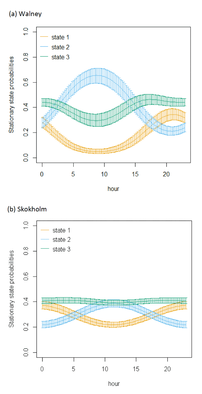
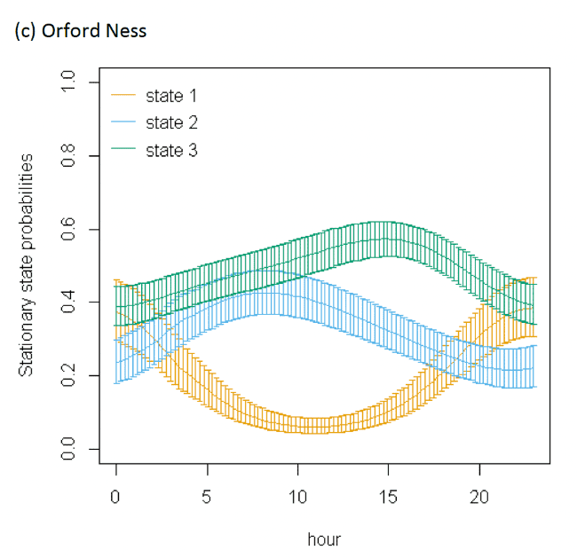
The best-fitting model, as assessed by AIC, was the full model with all covariates, being best across all colonies (Appendix AF). Transition and stationary state plots are show in Figure 8, Figure 9 and Appendix AD.

There were clear patterns over distance to colony for each of the three colonies modelled. These plots highlighted distances at which switches in behavioural states occurred from floating and foraging to commuting closer to colonies (as birds began travel to more distant feeding grounds), and then gradual switches to foraging/searching and floating away from commuting, presumably at foraging grounds (see Appendix AG). Over Julian date, there was also indication as the breeding season progressed that time spent floating at sea was reduced as birds transition to more searching and commuting activity – this may reflect birds having increasing breeding demands such as incubation and chick-rearing that required increasing amounts of foraging/searching activity and commuting to and from feeding locations (see Appendix AG).

The models showed very strong patterns over hour of the day (Figure 9). At all colonies, Lesser Black-backed Gulls were more likely to be floating on the sea during hours of darkness; a peak in floating activity was observed after 20:00 but the level of resting activity began to decrease after midnight, when transitions occurred from floating to foraging/searching and greater likelihood of remaining commuting. This resulted in clear peaks in commuting activity at the expense of other behaviours as seen in stationary state probabilities; however, the exact timing of peaks and troughs in foraging behaviour differed across colonies.

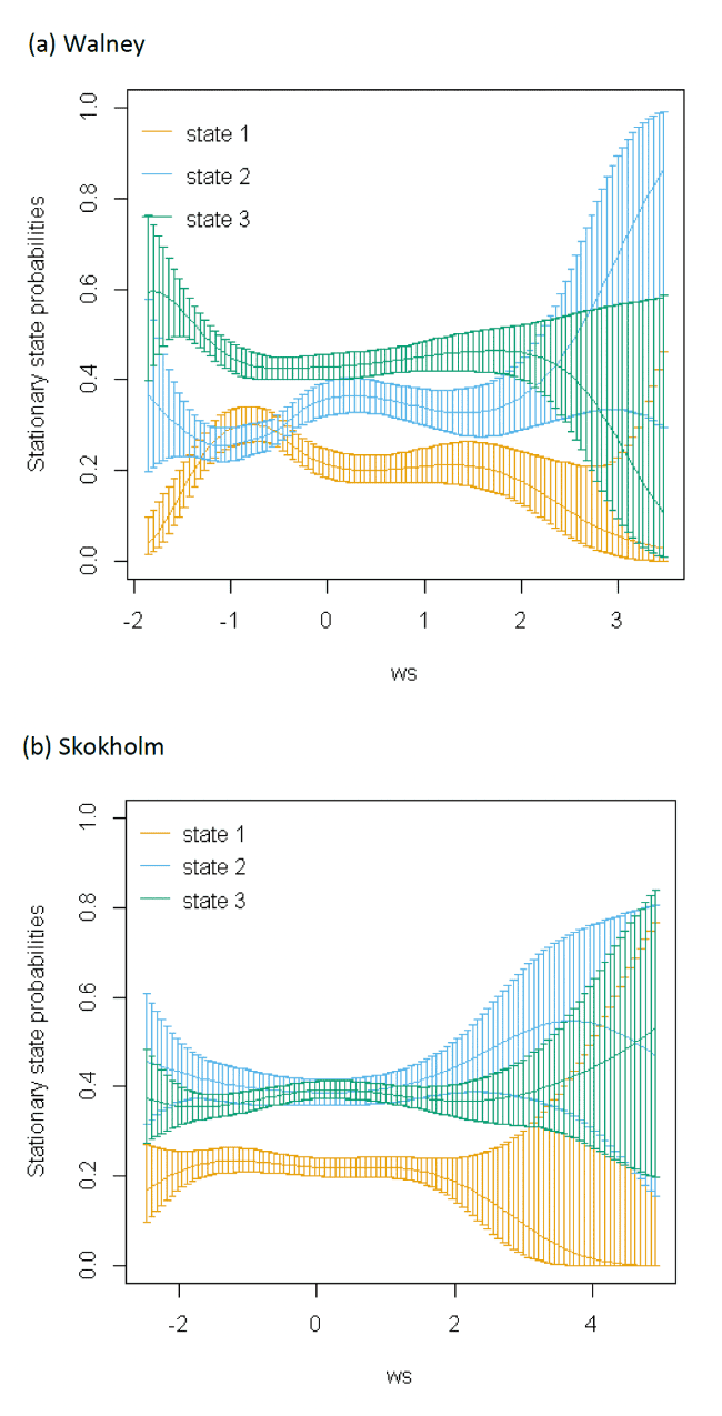
Models also indicated a complex pattern of transition probabilities between and within states over increasing wind speed (Figure 10). Patterns using the spline trends from the most parsimonious model (Appendix AF), were varied across colonies; for example, as wind speed increased, birds at Orford Ness spent less time resting and showed a greater tendency to switch from resting to foraging but wind speed had less effect on time spent resting at the other colonies. Noticeably at Walney, the likelihood of a fixes being commuting increased as wind speed increased. The effect of wind speed, however, was very closely linked with wind direction and the alignment of travel; hence all best-fitting models were significantly improved with this additional component added (dAIC >2.0), albeit as a linear effect rather than a spline.

When encountering headwinds birds were less likely to remain in the resting state and were more likely to transition from resting to foraging at Walney and Orford Ness. This pattern was not so apparent at Skokholm. However, at all colonies, the balance of remaining within and switching between different states yielded a similar stationary state probability over increasing wind speed, with reduced likelihood of floating over increasing wind speed, and increased likelihood of commuting. In headwinds, there was also an increased likelihood of birds remaining commuting and a clear increase in the time spent commuting over increasing wind speed in a headwind.

When viewed in terms of the strongest winds over the varying tail- and headwind spectrum of values (+1 to -1) patterns were similar over colonies; for Walney and Orford Ness, strong patterns of remaining in State 1 (floating) with a tailwind, and switching to State 3 (foraging/searching) in a headwind were observed, and for all colonies birds were less likely to remain commuting (2-2) and switch to foraging/searching with increasing tailwinds (2-3), being most similar between Walney and Skokholm. Consequently, stationary state probabilities were generally similar over colonies, with patterns of decreasing time spent commuting, and increasing foraging and floating over extent of tailwind alignment. Note however, that switches to foraging/searching from floating in headwinds were somewhat overshadowed within stationary state plots by the increasingly greater probability of commuting behaviour and birds being more likely to remain commuting when in headwinds.

3.2.6 Time in states

The range of duration of data per bird and the proportion of time spent in different states are shown in Table 12.

Table 12: For Lesser Black-backed Gull, estimated time spent in states for each colony for birds at each colony across years; note occasionally initial movement models could not be fitted due to a lack of data available for some individuals, hence the effective sample size feeding into assessments is provided in brackets.

			Duration of tracking			Proportion time spent per state
Colony	No. birds total (modelled)	Years	No. birds > 10 hrs tracking data	Duration (hrs) mean ± SD per bird	Tracking data range (hrs)	1 floating mean ± SD	2 commuting mean ± SD	3 foraging / searching mean ± SD
Walney	24 (22)	2014 to 2018	17	58.45 ± 120.11	1.67 – 497.42	0.20 ± 0.16	0.41 ± 0.22	0.39 ± 0.17
Skokholm	25 (25)	2014 to 2017	23	237.47 ± 183.88	3.8 – 270.4	0.32 ± 0.08	0.35 ± 0.13	0.35 ± 0.10
Orford Ness	24 (18)	2010 to 2015	17	90.80 ± 90.56	6.42 – 339.33	0.19 ± 0.15	0.39 ± 0.18	0.42 ± 0.08

3.2.7 Utilisation distributions

Figures depicting utilization distributions for each colony are shown in Appendix AH. Depending on the colony, there was a smaller amount of data from the very highest wind speeds (greater than 8 m/s) – see methods, and also section above comparing use and availability for wind speed distributions.

Low sample sizes were recorded for the day-high category for the floating state at Walney, with less than three birds and only 78 fixes providing data. For Orford Ness, low sample sizes of only two birds and 49 fixes were obtained for the day-high category for the same floating state, and further, only four birds provided data for the night-high floating state. These data should be treated with caution, and are highlighted in plots with red borders around utilisation distribution maps. We again also caution the comparison of utilisation distributions based on very disparate numbers of fixes. For Lesser Black-backed Gulls at all colonies, a number of high and low wind categories (day and night) represented less than 5% of the number of fixes available, and was found across all three states.

3.2.8 Overlap indices

Overlaps between states in different conditions and times of the day are visualized in Appendix AI, and summarised in Table 13.

For Lesser Black-backed Gulls across all colonies, the 95% KDEs, representing total area usage, generally showed a moderate (BA = 0.4-0.6) to very high (BA = 0.8+) level of overlap, between the daytime low-wind conditions (taken here as representative of similar conditions that aerial surveys would encounter), and the other scenarios of day-high wind, night-low wind and night-high wind scenarios across different states; the exception to this was the resting State 1 for Walney (BA = 0.37). At all colonies, the greatest overlaps were between day-low and day-high wind for the state of commuting (BA = 0.84, 0.90 and 0.90 for each colony, respectively), suggesting commuting zones used were not noticeably different during the day in different wind conditions. Overlaps between the core (50% KDE) day-low and other conditions were lower than the total 95% KDE for all states. Overlaps were generally lowest for the comparison of day-low vs night-high across colonies, and were again most pronounced for the State 1 floating, however, the smallest overlap index (BA = 0.06) was seen for day low vs day high floating at Walney.

We found that overlaps for the night-high vs night-low comparison were lower than day-high vs day-low comparisons across states (Table 13). There were also similar magnitudes of difference when comparing day-low and night-low and day-high and night-high; overlap indices were higher (for 95% and 50% KDEs) between day and night in low wind conditions, than comparing day and night in high wind conditions, which was true across all states. Birds at all colonies often rested just offshore (close to the colony) on the sea overnight, which was not done so during the day, however, during both day and night birds rested on the sea offshore during day and night periods. In generalising, these results may indicate similar magnitudes of drivers of wind speed than time of day for distributions for Lesser Black-backed Gulls but again overall overlaps in distributions are generally considered moderate to very high for this species.

Table 13: For Lesser Black-backed Gull, overlap indices (Bhattacharyya's Affinity Index) for pair-wise combinations of utilisation distribution assessing similarity in 95% KDEs (and 50%, brackets) for different levels of day and night, and high/low wind and states 1, 2 and 3 (floating, commuting and foraging/searching); bold highlights indicate comparisons of greatest interest, comparing the equivalent conditions when surveys are made (low wind daytime) to other conditions; red highlight shows where confidence in overlap assessment is lowest due to low sample sizes (see methods and Appendix AA).

(a) Walney

state		day.high	day.low	night.high
1	day.low	0.37 (0.06)
1	night.high	0.17 (0)	0.37 (0.08)
1	night.low	0.32 (0)	0.59 (0.29)	0.38 (0.08)
2	day.low	0.84 (0.6)
2	night.high	0.68 (0.46)	0.68 (0.42)
2	night.low	0.79 (0.5)	0.88 (0.6)	0.87 (0.68)
3	day.low	0.72 (0.5)
3	night.high	0.58 (0.06)	0.55 (0.12)
3	night.low	0.68 (0.27)	0.82 (0.54)	0.69 (0.27)

(b) Skokholm

state		day.high	day.low	night.high
1	day.low	0.77 (0.46)
1	night.high	0.47 (0.19)	0.56 (0.28)
1	night.low	0.53 (0.21)	0.72 (0.39)	0.48 (0.22)
2	day.low	0.9 (0.85)
2	night.high	0.75 (0.66)	0.81 (0.7)
2	night.low	0.84 (0.74)	0.92 (0.84)	0.8 (0.69)
3	day.low	0.85 (0.56)
3	night.high	0.51 (0.09)	0.57 (0.24)
3	night.low	0.67 (0.18)	0.8 (0.35)	0.62 (0.36)

(c) Orford Ness

state		day.high	day.low	night.high
1	day.low	0.47 (0.45)
1	night.high	0.38 (0.17)	0.4 (0.14)
1	night.low	0.39 (0.26)	0.6 (0.37)	0.43 (0.26)
2	day.low	0.9 (0.84)
2	night.high	0.61 (0.32)	0.63 (0.33)
2	night.low	0.87 (0.79)	0.92 (0.9)	0.64 (0.36)
3	day.low	0.71 (0.59)
3	night.high	0.54 (0.39)	0.5 (0.22)
3	night.low	0.64 (0.53)	0.77 (0.43)	0.47 (0.21)

3.3 Black-legged Kittiwake

3.3.1 Comparison of wind speed use vs availability

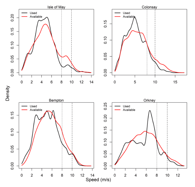
Comparisons of wind speeds experienced and those available within the grid cells of the Copernicus weather data that birds overlapped with offshore were made for all colonies – see Table 14, Figure 11 and Appendix AB.

For all colonies except Colonsay, precise periods where individual birds were tracked percentages were lower than that of the entire month. The use, however, as recorded through wind speeds experienced at GPS fixes, revealed lower proportions of 8 m/s and 10 m/s data compared to that available during the same period of tracking. Birds at Colonsay and Orkney also showed a higher proportion of high wind speed data than Isle of May and Bempton, being northerly and westerly in location.

Table 14: For Kittiwake, summary of the proportions of tracking data by wind speed thresholds of more than 10 m/s and more than 8 m/s, and further comparing wind speeds encountered by birds ('used') vs wind speeds 'available'. Assessment is made both (i) within the full months that tracking was carried out and (ii) for the precise tracking date-times, for all Copernicus grid squares that birds overlapped with; proportions for 'use' data are calculated on the data modelled within HMMs, thus each data point is a GPS fix; for 'available' calculations, each data point is an hourly wind speed estimate for each Copernicus grid square.

		Used (%)		Available (tracking period, %)		Available (all months, %)
Colony / State	Tracking months and years	8 m/s	10 m/s	8 m/s	10 m/s	8 m/s	10 m/s
Isle of May	May – July, 2012 – 2014	6.72	1.71	13.94	3.11	18.57	6.2
Colonsay	June – July, 2010 – 2014	14.57	4.35	21.86	9.91	18.5	7.06
Bempton Cliffs	June – July, 2010 – 2015	12.24	2.93	16.29	3.66	21.65	7.29
Orkney	June – July, 2010 – 2014	13.88	3.07	20.37	6.02	23.77	7.91

3.3.2 Model summary

Three-state model

For each colony, mean step lengths (from gamma distribution) and angle parameters (mean and concentration from Von Mises) for each state are shown in Table 15 below. Together these models indicated more consistent direction for slower floating on the sea State 1 and faster commuting State 2, in contrast to State 3 with wider turning angles and a lower consistency in direction between fixes (Appendix AC).

Table 15: Summary of mean ± SD step length and turning angles (mean, concentration) for each site.

	Step			Turn
Colony / State	1 (floating)	2 (commuting)	3 (forage/ search)	1 (floating)	2 (commuting)	3(forage/ search)
Isle of May	48.37 ± 20.39	1066.33 ± 355.12	176.51 ± 193.25	0, 8.65	0, 8.26	0, 0.41
Colonsay	56.95 ± 36.92	1087.81 ± 383.62	144.07 ± 186.63	0, 13.29	0, 8.26	0, 0.19
Bempton Cliffs	59.73 ± 28.41	1239.50 ± 317.34	262.19 ± 297.57	0, 21.70	0, 26.33	0, 0.70
Orkney	105.80 ± 88.67	1020.85 ± 437.68	98.62 ± 139.30	0, 12.72	0, 40.50	0, 0.28

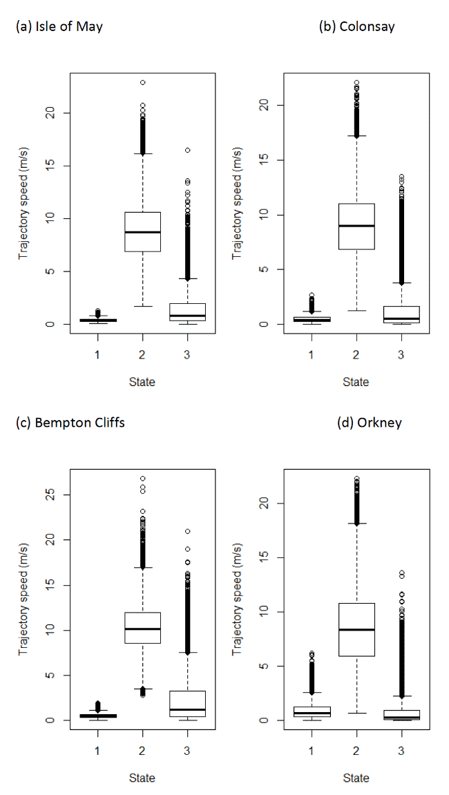
At all colonies, direct transitions to and from States 1 (floating) and 2 (commuting) were typically rarer in the datasets, as also found in some other studies (see Dean et al. 2013). Most frequently, fixes following a particular state were most likely to be classified as the same state again. However, where switches did occur, typically floating on the sea was preceded and succeeded by locations classified as State 3, with further switches occurring between commuting and foraging (Appendix AC).

Four-state model

Four-state models indicated that a further stationary state could be identified from the datasets, that aimed to represent birds perching at sea or on land away from the breeding colony, or other behaviours such as preening or social interactions on the sea surface when not in flight. Comparing this model to the three state model, generally involved differing classifications of the "foraging/searching" and "floating on sea" states from the three state model; note, commuting was more consistently classified between three and four state models.

For example, for the Isle of May, a four-state model gave mean step lengths for each state as 61.69 ± 52.32, 49.20 ± 17.04, 1156.47 ± 318.38 and 433.15 ± 295.74 for "stationary floating", "floating on the sea", "commuting" and "foraging/searching respectively" (States 1-4 for the four-state approach), with concentration parameters for the von Mises angle distribution given as 0.55, 16.78, 14.58 and 0.89 for each state respectively. Thus as with the three-state model, commuting and floating on the sea had more consistent direction, differing by speed distinctions, and similarly, slow potential perching behaviour had similar wide turning angles between fixes, t and t + 1, differing in speed delineations.

3.3.3 Travel speeds

Three-state model

The HMMs can be used to estimate travel speeds in each state (Figure 12). Table 16 below shows the distributions of speeds from boxplot analysis after assigning states back to the raw data. The behaviour of "foraging/searching" identified from HMMs, although encompassing behaviours associated with foraging at or near the sea surface at very slow speeds including potentially not being in flight, could also encompass some stationary activity, for example if birds perch on structures at sea, or around coastlines when away from the colony. Four-state models were, therefore, also specified for investigation of potential behaviours that were slower and that had wide-turning angles, thus simulating possible floating in a single location or bathing activity on the sea surface – see below.

Table 16: For Kittiwake, summary of speeds per state (m/s), as obtained through classification of tracking data using three-state HMMs.

Colony / State	1 (floating)	2 (commuting)	3 (forage/search)
Isle of May	0.39 (0.29 – 0.49)	8.69 (6.91 – 10.61)	0.78 (0.31 – 1.92)
Colonsay	0.38 (0.25 – 0.62)	8.97 (6.87 – 11.00)	0.49 (0.13 – 1.60)
Bempton Cliffs	0.47 (0.33 – 0.63)	10.17 (8.54 – 11.92)	1.15 (0.40 – 3.24)
Orkney	0.64 (0.36 – 1.24)	8.35 (5.89 – 10.79)	0.26 (0.05 – 0.93)

Four-state model

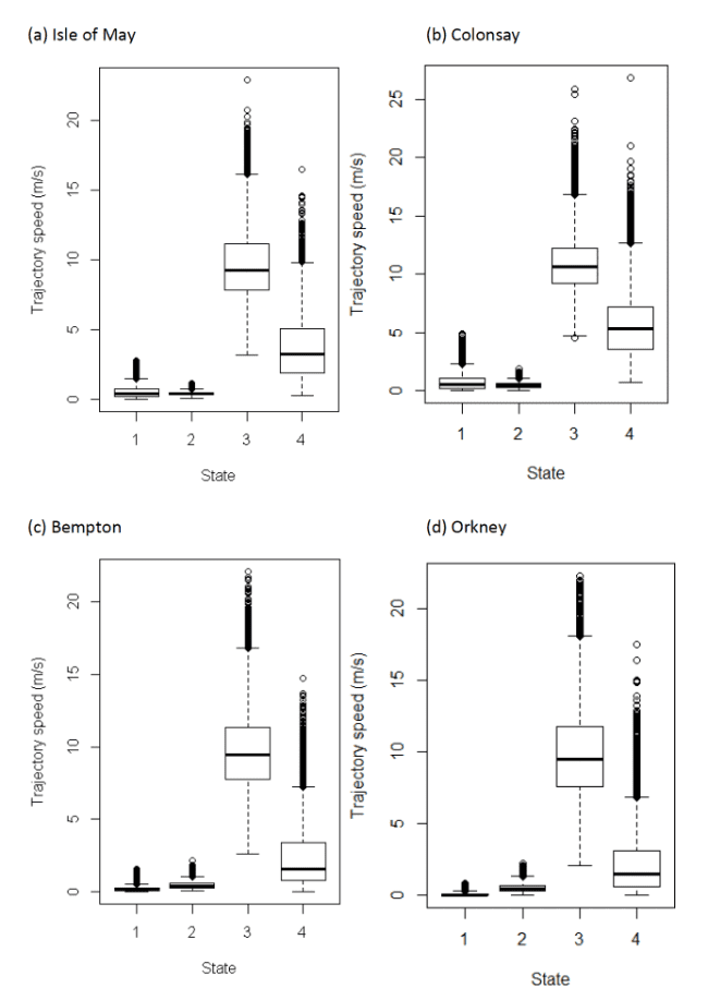
Four-state HMMs estimated that a further stationary state could be identified (Table 17), and generally involved differing classifications of the "foraging/searching" and "floating on sea" states from the three state model (see Table 16); note, commuting was more consistently classified between three and four state models.

Table 17: For Kittiwake, estimated median (lower quartile – upper quartile trajectory speeds for each site, as obtained through classification of GPS fixes by HMM States (1-3).

Colony / State	1 (perching)	2 (floating)	3 (commuting)	4 (forage/search)
Isle of May	0.41 (0.20 – 0.72)	0.39 (0.31 – 0.49)	9.26 (7.82 – 11.14)	3.21 (1.86 – 5.05)
Colonsay	0.12 (0.05 – 2.47)	0.40 (0.28 – 0.60)	9.45 (7.76 – 11.37)	1.56 (0.78 – 3.36)
Bempton Cliffs	0.55 (0.24 – 1.09)	0.48 (0.34 – 0.63)	10.61 (9.20 – 12.27)	5.37 (3.57 – 7.21)
Orkney	0.05 (0.02 – 0.13)	0.48 (0.31 – 0.72)	9.52 (7.59 – 11.78)	1.50 (0.63 – 3.13)

This analysis revealed a greater speed for "foraging/searching" speed for each colony respectively than the three-state model for "foraging/searching" (see above); the four-state model also varied between colonies in the speed for this category (Figure 13). The four-state delineation for "foraging/searching" is likely more indicative of inflight behaviour, however, conversely it is not possible to rule out activity that is within the three-state model "foraging/searching" category that is also non-flight activity related to foraging, such as on-the-sea activity.

3.3.4 Effects of wind speed on step length (speed)

For all further analyses, the three-state model was used to investigate effects of covariates.

For all colonies, there was a distinct effect of wind speed in on travel speeds for commuting that further varied by whether wind direction was aligned with travel direction of the bird (Appendix AE) - a positive value was recorded for the interaction effect of wind speed:angle_osc coefficient (Isle of May, β = 0.507, Colonsay 0.408, Bempton Cliffs, β = 0.490 m and Orkney β = 0.407). Thus, faster commuting speeds were recorded in faster wind speeds that were in turn aligned with the direction of travel of the bird (i.e. tailwinds), as given through the angular_osc covariate (-1 = headwind, +1 = tailwind). At all colonies, there was little influence of birds aligning turning angles during commuting with prevailing wind directions, i.e. turning with the wind (Isle of May, β = -0.021, Colonsay β =-0.022, Bempton Cliffs, β = -0.002, Orkney β = -0.058), being perhaps unsurprising as birds make outward and return movements often against the wind.

3.3.5 Transition effects between states in relation to covariates

Across all colonies, the best fitting models was the full model containing all covariates (Appendix AF). Transition and stationary state probability plots are presented in Figure 14, Figure 15 and Appendix AD.

There were clear associations between behavioural state and distance from the colony (Appendix AD). For example, distances can be identified at which switches in behavioural states occurred from floating and foraging to commuting close to colonies (as birds began travel to more distant feeding grounds), and then gradual switches to foraging/searching and floating away from commuting, presumably at foraging grounds (see Appendix AG). The relationship between behavioural states and Julian date varied across colonies (see Appendix AG) and are difficult to reliably compare due to different periods of study for each colony and are also hard to appreciate without further scrutiny of egg and chicks stage analyses, thus here serving mainly as a control variable.

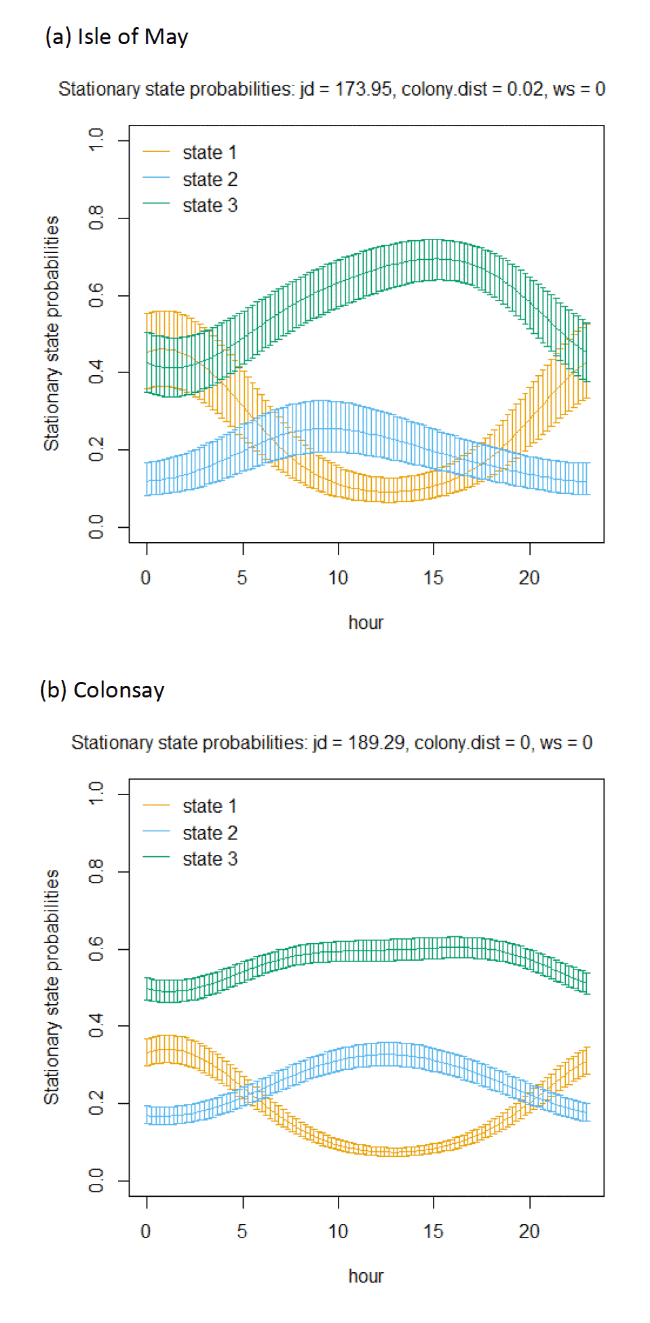
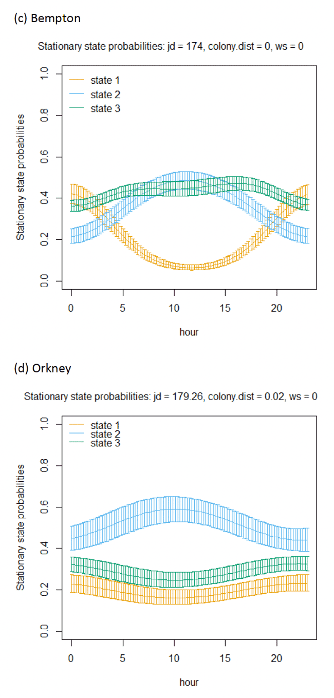
In terms of the aims of this project, the models for all colonies showed strong diurnal patterns in behaviour, but naturally also dependent on the amount of daylight across the season (Figure 14). At all colonies, Kittiwakes, were more likely to be floating on the sea during hours of darkness; the spline model (df = 4) indicated a gradual reduction of floating activity from ca. 00:00 – 03:00 until ca. 09:00 – 15:00 when floating was at its lowest and birds were most active in flight at sea. As noted above, transitions between States 1 and 2 were uncommon, and thus patterns of commuting were informed by likelihood of remaining commuting or transitioning to and from foraging/searching activity; switches between floating and foraging indicated birds at all colonies were more likely to transition to foraging/searching (State 3) later in the day (e.g. ca. 10:00 – 20:00), most apparently for Isle of May and Colonsay.

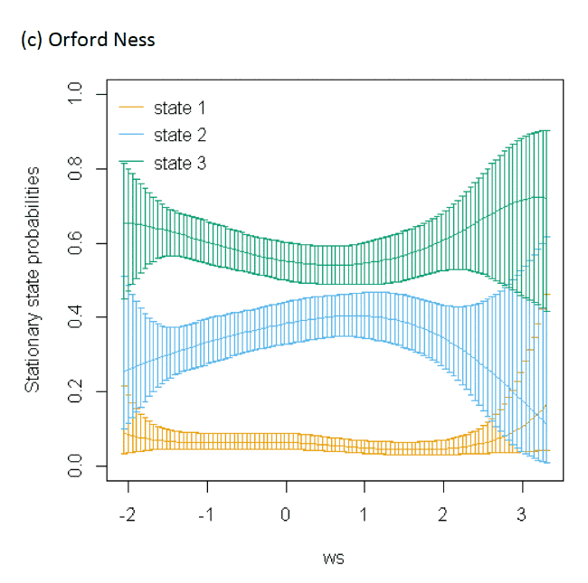
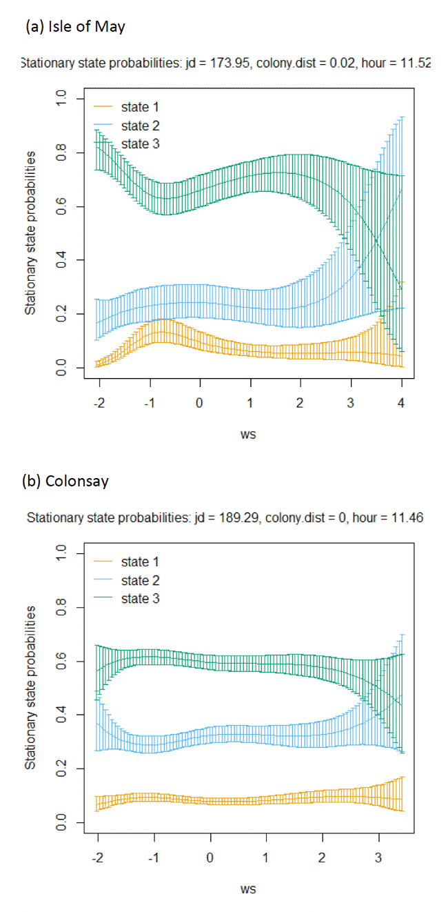
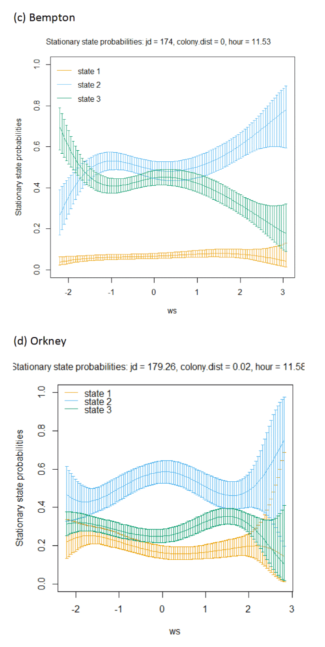
Models also indicated a complex pattern over increasing wind speed (Figure 15). At the Isle of May, Kittiwakes were more likely to transition from floating on the sea surface to searching/foraging as wind speed increased, although not at the very lightest or strongest winds, but with more error at this point in the curve. For Colonsay, likewise there were complexities in the spline relationship but overall there were decreases in probabilities for remaining floating over increasing wind speed, and swicthes to foraging, this time at the fastest wind speeds. For Bempton Cliffs, shapes of the splines for transitions 1-1 and 1-3 were similar to the Isle of May, albeit less pronounced. At all colonies, the probability of birds remaining in the commuting state increased as wind speed (was positively associated with wind speed), partly also reflected in stationary state probability plots.

Examining wind speed patterns more closely through interaction with headwinds and tailwinds (wind speed x angle_osc parameter) and modelling wind speed as a linear term rather than a spline, revealed some clearer relationships. At the Isle of May, birds were less likely to remain in the resting state and more likely to switch from resting to foraging with increasing tailwind speeds. A similar, although shallower trends in relationships was shown for Bempton Cliffs, and even less so for Colonsay. At all colonies, birds were less likely to persist in the foraging state but more likely to persist in the commuting state as tailwind speed increased, reflected in the stationary state plots. Patterns of state likelihoods across colonies showed greater parity when viewed at the fastest wind speeds at each site, and examined across the spectrum of tail, cross and headwind (+1 to -1) spectrum for the angle_osc variable. At all colonies, birds were more likely to switch from floating to foraging as birds encountered headwinds rather than tailwinds, and vice versa. Further, birds were more likely to remain commuting in headwinds, and switch from commuting to foraging/searching over increasing tailwinds.

3.3.6 Time in states

The range of duration of data per bird and the proportion of time spent in different states are shown in Table 18. As birds with fewer data had less time to demonstrate their overall time spent in different states, we used information from birds with more than ten hours of data, to exclude any very small tracking durations that could otherwise skew patterns observed.

Table 18: For Kittiwake, estimated time spent in states for each colony for birds at each colony across years; note occasionally initial movement models could not be fitted due to a lack of data available for some individuals, hence the effective sample size feeding into assessments is provided in brackets.

		Duration of tracking				Proportion time spent per state
Colony	No. birds total (modelled)	Years	No. birds > 10 hrs tracking data	Duration (hrs) mean ± SD per bird	Tracking data range (hrs)	1 floating mean ± SD	2 commuting mean ± SD	3 foraging / searching mean ± SD
Isle of May	50 (49)	2012 to 2014	33	21.92 ± 9.47	4.3 – 50	0.22 ± 0.09	0.25 ± 0.07	0.53 ± 0.10
Colonsay	84 (81)	2010 to 2014	81	32.58 ± 18.34	3.57 – 97.13	0.20 ± 0.10	0.26 ± 0.12	0.55 ± 0.12
Bempton Cliffs	104 (97)	2010 to 2015	81	28.97 ± 16.96	0.3 – 89.4	0.22 ± 0.10	0.30 ± 0.10	0.47 ± 0.11
Orkney*	86 (80)	2010 to 2014	64	21.91 ± 8.55	0.8 – 42.1	0.17 ± 0.09	0.28 ± 0.17	0.55 ± 0.18

* = data for Orkney from Copinsay and Muckle Skerry combined

3.3.7 Utilisation distributions

Figures depicting utilization distributions for each colony are shown in Appendix AH. Depending on the colony, there was a smaller amount of data from the very highest wind speeds (greater than 8 m/s) – see also section above comparing use and availability for wind speed distributions.

For Kittiwakes, low sample sizes were primarily an issue for the Isle of May and centered around the number of birds available under high wind conditions; the day-high floating state was based on only two birds (103 fixes); the night-high category had less than or equal to five birds providing data for all states, and the commuting state had only 45 fixes. These categories should thus be treated with a high degree of caution, with less confidence placed in the final overlap assessments based on these data. For other colonies, in each category and state, there were more than five birds and more than 100 fixes, however, night-high categorisations at all colonies for the states of commuting and foraging represented less than 5% of the total data available. We again also caution the comparison of utilisation distribution based on very different numbers of GPS fixes.

3.3.8 Overlap indices

Overlaps between states in different conditions and times of the day are visualized in Appendix AI, and summarised in Table 19.

For Kittiwakes at all colonies, the 95% KDEs, representing total area usage, showed generally moderate (BA = 0.4 – 0.6) to very high (BA = 0.8+) levels of overlap, between the daytime low-wind conditions (taken here as representative of similar conditions that aerial surveys would encounter), and the other scenarios of day-high wind, night-low wind and night-high wind scenarios across different states; the exception to this was for the Isle of May and Bempton Cliffs night-high floating State 1 pair-wise test (BA = 0.34 in both cases), and also the night-high comparison for Bempton Cliffs for the foraging/searching State 3 (BA = 0.34).

At all colonies, a high (BA = 0.6 – 0.8) degree of overlaps was seen across colonies between day-low and day-high wind for the state of commuting, suggesting (generally) commuting zones used were not noticeably different during the day in different wind conditions. This wasn't fully the case however, with moderate overlaps with day-low and night-high for the Isle of May and Bempton commuting State 2 (BA = 0.43 and 0.51). Overlaps between the core (50% KDE) day-low and other conditions were lower than the total 95% KDE for all states, and generally reflected the same patterns above for total area use. Comparing day-low with the other three conditions, some notably very low overlaps in the core 50% KDEs were recorded for the day-low vs nigh high at three colonies, Colonsay, Bempton and Orkney, with low overlaps for Isle of May (BA = 0.28, 0.17, 0.15 and 0.07) – this comparison, therefore, represents the most extreme difference of the four-way paired tests, but note that sample sizes for night-high wind conditions was lowest of all categorisations of data.

On inspection, the overlaps for the night-high vs night-low comparison were lower than day-high vs day-low comparisons across states, and these difference in BA indices were similar in magnitude to comparisons of day-low and night-low and day-high and night-high (Table 19). There were therefore some clear differences in overlaps across times of day and conditions that in turn varied between different states, and further variation between colonies, making drawing general conclusions difficult. For example, there was an indication for Isle of May and Colonsay that some areas further offshore were not used for floating on the sea (floating) during higher wind conditions (but noting reduced high wind speed sample sizes). However, given that many BA indices were classed as 'moderate' and above for 95% and 50% KDE comparisons, a general conclusion may be that space use overall can be considered similar across day-night and high and low wind.

Table 19: For Kittiwake, overlap indices (Bhattacharyya's Affinity Index) for pair-wise combinations of utilisation distribution assessing similarity in 95% KDEs (and 50%, brackets) for different levels of day and night, and high/low wind and states 1, 2 and 3 (floating, commuting and foraging/searching); bold highlights indicate comparisons of greatest interest, comparing the equivalent conditions when surveys are made (low wind daytime) to other conditions; red highlight shows where confidence in overlap assessment is lowest due to low sample sizes (see methods and Appendix AA).

(a) Isle of May

state		day.high	day.low	night.high
1	day.low	0.46 (0.21)
1	night.high	0.33 (0.05)	0.34 (0.28)
1	night.low	0.28 (0.04)	0.52 (0.29)	0.31 (0.15)
2	day.low	0.62 (0.56)
2	night.high	0.54 (0.37)	0.43 (0.29)
2	night.low	0.59 (0.6)	0.72 (0.65)	0.53 (0.41)
3	day.low	0.59 (0.48)
3	night.high	0.6 (0.41)	0.48 (0.39)
3	night.low	0.48 (0.33)	0.71 (0.58)	0.52 (0.41)

(b) Colonsay

state		day.high	day.low	night.high
1	day.low	0.61 (0.67)
1	night.high	0.59 (0.37)	0.44 (0.17)
1	night.low	0.51 (0.51)	0.66 (0.58)	0.45 (0.19)
2	day.low	0.73 (0.74)
2	night.high	0.68 (0.69)	0.6 (0.63)
2	night.low	0.7 (0.67)	0.83 (0.72)	0.62 (0.62)
3	day.low	0.72 (0.72)
3	night.high	0.7 (0.55)	0.54 (0.4)
3	night.low	0.68 (0.72)	0.81 (0.76)	0.56 (0.46)

(c) Bempton Cliffs

state		day.high	day.low	night.high
1	day.low	0.47 (0.28)
1	night.high	0.48 (0.38)	0.34 (0.15)
1	night.low	0.49 (0.35)	0.63 (0.45)	0.36 (0.19)
2	day.low	0.8 (0.58)
2	night.high	0.63 (0.38)	0.51 (0.32)
2	night.low	0.77 (0.62)	0.82 (0.79)	0.56 (0.43)
3	day.low	0.57 (0.37)
3	night.high	0.49 (0.35)	0.32 (0.03)
3	night.low	0.51 (0.37)	0.75 (0.68)	0.39 (0.09)

(d) Orkney

state		day.high	day.low	night.high
1	day.low	0.74 (0.77)
1	night.high	0.48 (0.06)	0.47 (0.07)
1	night.low	0.36 (0.38)	0.61 (0.45)	0.38 (0.13)
2	day.low	0.69 (0.7)
2	night.high	0.66 (0.33)	0.56 (0.46)
2	night.low	0.53 (0.54)	0.72 (0.68)	0.57 (0.51)
3	day.low	0.87 (0.9)
3	night.high	0.83 (0.92)	0.82 (0.93)
3	night.low	0.75 (0.89)	0.86 (0.97)	0.79 (0.93)

3.4 Razorbill

3.4.1 Comparison of wind speed use vs availability

Comparisons of wind speeds experienced and those available within the wider area were made for all colonies – see Table 20 and Figure 16 and Appendix AB.

For Razorbills at Colonsay and Puffin Island, similar availability percentages were obtained when using data from the full months of tracking and the precise periods where individual birds were tracked within these months. For the Isle of May, windier conditions were experienced during tracking periods than across the months of tracking. Correspondingly, the use of wind speeds by birds at the Isle of May was disproportionally higher than that available across the month, but not in comparison to available within the tracking period, and all proportions over 10 m/s was lower for conditions birds actually experienced vs that available. The conditions that birds experienced at Colonsay, revealed slightly lower but similar percentages to availability percentages, however, for Puffin Island, lower 'use' percentages were recorded. In comparison to Colonsay, Puffin Island wind speeds over the squares utilised by birds were windier, yet similar proportions of 'use' wind speeds were found at both sites, providing potential indication that Razorbills may have not selected stronger winds at Puffin Island to the extent at which they were available Razorbill. These findings may be attributable to the shorter foraging ranges at Puffin Island, meaning that windier conditions offshore are not used, in turn making it harder to assess how birds at this colony respond to windier conditions. Such colony-specific variations are therefore apparent, and may be further complicated by some individuals at some colonies struggling to find enough prey for chicks and thus having to travel further (in turn experiencing windier conditions offshore).

Table 20: For Razorbill, summary of the proportions of tracking data by wind speed thresholds of more than 10 m/s and more than 8 m/s, further comparing wind speeds encountered by birds ('used') vs wind speeds 'available'. Assessment is made both (i) within the full months that tracking was carried out and (ii) for the precise tracking date-times, for all Copernicus grid squares that birds overlapped with; proportions for 'use' data are calculated on the data modelled within HMMs, thus each data point is a GPS fix; for 'available' calculations, each data point is an hourly wind speed estimate for each Copernicus grid square.

		Used (%)		Available (tracking period, %)		Available (all months, %)
Colony / State	Tracking months and years	8 m/s	10 m/s	8 m/s	10 m/s	8 m/s	10 m/s
Isle of May	June – July 2012, June 2013, 2014	12.31	0.48	16.23	3.3	7.07	1.34
Colonsay	July 2010, June – July 2011 – 2014	14.9	3.99	15.83	4.96	15	4.69
Puffin Island	May – June, 2011; June 2013; May 2012, 2015	11.91	3.92	23.64	11.19	27.46	11.62

3.4.2 Model summary

The best fitting models corresponding to Razorbills tagged on Colonsay, Puffin Island, and the Isle of May are presented in Appendix AF. Table 21 displays the step lengths and angle concentrations corresponding to the three behavioural states in relation to each study site. In general, State 1 (floating) and State 2 (commuting) contained obtuse turning angles, with step lengths being relatively short in State 1, and longer in State 2. State 3 (foraging) exhibited acute turning angles and the shortest relative step lengths (Appendix AC).

Table 21: For Razorbill, summary of mean ± SD step length and turning angles (mean, concentration) for each site.

	Step			Turn
Colony / State	1 (floating)	2 (commuting)	3 (forage/ search)	1 (floating)	2 (commuting)	3 (forage/ search)
Colonsay	41.33 ± 21.64	806.16 ± 837.69	18.81 ± 17.00	0, 17.16	0, 2.01	0, 0.06
Puffin Island	79.87 ± 32.49	768.72 ± 816.18	21.67 ± 19.98	0, 107.09	0, 2.21	0, 0.82
Isle of May	39.88 ± 18.15	648.27 ± 843.31	11.42 ± 10.02	0, 7.46	0, 0.67	0, 0.01

Razorbills from Colonsay transitioned between floating (States 1) and commuting (State 2) less frequently than transitions between floating to foraging (State 3) (Appendix AC). In contrast, individuals from Puffin Island and the Isle of May transitioned proportionately more frequently from floating (State 1) to commuting (State 2) than floating to foraging (State 3). State changes from foraging to floating occurred more frequently than transitions from foraging directly to commuting at all three study sites. These relationships are proportionally less in Razorbills from Puffin Island than from Colonsay or the Isle of May, with no clear trends between state transitions (Appendix AC). Razorbills from all three colonies exhibited strong tendencies to remain within their previous states. With regards to Razorbills from Colonsay, the tendency for birds to remain foraging was weaker than Colonsay or the Isle of May, this potentially contributed to a lack of discernible trends in state transitions on Puffin Island.

For Colonsay, the model incorporating an additional dive depth parameter displayed some differing transition probabilities in comparison to the model excluding diving (Appendix AC). Primarily, the proportional transition from float to commute was much more pronounced, with the probability of remaining floating reduced. The probability of a foraging state transitioning to floating or commuting remained similar, although the probability of remaining in a foraging state increased.

Time-depth recorder (TDR) data was available for sub-sample of concurrently GPS tracked individuals (n = 25, Colonsay). The proportion of dives > 5 m used as a third covariate alongside turning angle and step length within HMMs. Table 22 displays the step lengths and angle concentrations corresponding to the three behavioural states in relation to each study site, using the best-fitting model (Appendix AF).

Table 22: For Razorbills, summary of mean ± SD step length and turning angles (mean, concentration) for Colonsay based on HMMs using both GPS and TDR data.

	Step			Turn
Colony / State	1 (floating)	2 (commuting)	3 (forage/search)	1 (floating)	2 (commuting)	3 (forage/search)
Colonsay	35.8 ± 20.38	151.34 ± 254.66	201.66 ± 253.57	0, 13.05	0, 0.12	0, 1.59

The proportion of dives per GPS fix that were classified as belonging to different States (1-3) are given in Table 23 below. These comparisons acted as a post-hoc verification of the classifications using TDR data through the HMM model with the additional channel of dive depth; these results indicate that the foraging/searching state contained the most GPS fixes that were identified from the model as being both in the state "foraging/searching" and being beneath the water, i.e. dives indeed did fall within the foraging/searching category.

Table 23: For Razorbills, total number of GPS fixes for states 1, 2 and 3 (floating, commuting and foraging/searching) categorised by the proportion of time spent deeper than 5 m at Colonsay.

Dive proportion category	State 1 (floating)	State 2 (commuting)	State 3 (foraging/searching)
0	16427	32318	0
0 – 0.5	14	403	1341
0.5 – 1.0	12	1	94

We also investigated the corresponding classification of GPS points between the non-TDR (standard HMM with no dive depth channel included) and TDR HMMs (including the additional dive channel). This comparison was conducted on the subset of Razorbills at Colonsay that were included in both analyses, and for each GPS fix, assessing the state assignment between the two approaches. Table 24 below shows this comparison and indicated that although there was a good match for the floating State 1, there was considerably more discrepancy between commuting State 2 and the foraging/searching State 3. In particular, the standard HMM most often assigned a foraging state, which for the TDR models was classified mostly as commuting. These discrepancies are perhaps testimony to the difficulty of applying HMMs to these species, which requires further work to fully resolve. These discrepancies, however, were less apparent in spatial plots comparing the distribution of states (Appendix AC) Further, the HMMs also classified some points as resting on the sea for commuting (see the strings of red aligned points, i.e. at lower speed, to the bottom right of the images), with potential consequences for interpretation of commuting speed for this species.

Table 24: For Razorbill, total number of GPS fixes corresponding in behavioural states 1, 2 and 3 (floating, commuting and foraging/searching) between Non- TDR and TDR incorporating models for Colonsay.

TDR
	States	1	2	3
Non-TDR	1	12693	581	543
	2	87	5010	378
	3	3673	27131	514

3.4.3 Travel speeds

Table 25 below shows the distributions of speeds from boxplot analysis (Figure 17) after assigning states back to the raw data and birds modelled using the additional TDR dive variable (Figure 18). It is likely that the foraging state encompassed bouts of diving, in which birds will move only negligible distances between GPS fixes. The influence of diving on the outcome of the models was also investigated in Guillemots, where TDR data was available for a subsample of birds.

Table 25: For Razorbills, summary of speeds per state (m/s), as obtained through classification of tracking data using HMMs.

Colony / State	1 (floating)	2 (commuting)	3 (forage/search)
Standard model
Colonsay	0.37 (0.26 – 0.53)	3.62 (1.34 – 14.44)	0.13 (0.06 – 0.25)
Puffin Island	0.77 (0.56 – 1.01)	4.75 (1.10 – 14.23)	0.15 (0.06 – 0.28)
Isle of May	0.36 (0.27 – 0.47)	1.50 (0.65 – 12.03)	0.07 (0.04 – 0.15)
TDR data included
Colonsay	0.31 (0.21 – 0.47)	0.15 (0.06 – 0.41)	0.51 (0.28 – 0.88)

3.4.4 Effects of wind speed on step length (speed)

Step lengths relating to specific states were plotted over increasing wind speeds for Colonsay, Puffin Island and Isle of May (Appendice AD and AE). Colonsay Razorbills exhibited a decrease in floating (State 1) and foraging (State 3) step lengths in relation to increasing wind speeds (β = -0.048, β = -0.012). Conversely, step lengths in the commuting state (State 2) were positively associated with wind speed (β = 0.0069) at Colonsay. Wind speed maintained a positive relationship with increasing step lengths across all states at Puffin Island state 1 (β = 0.033), state 2 (β = 0.023), and state 3 (β = 0.055). With regards to the Isle of May Razorbills, step length exhibited a decreasing relationship with increasing wind speeds in in relation to State 1 (β = -0.027) and 2 (β = -0.014), but displayed a weak positive relationship in state 3 (β = 0.0017).

3.4.5 Transition effects between states in relation to covariates

AIC selection indicated the best-fitting model, for both Colonsay, Puffin Island, and the Isle of May contained all the covariates (hour + Julian date + colony distance + wind speed) (Appendix AF). The best-fitting model selected for Colonsay, when incorporating dive depth variable, retained only 'hour'.

At each colony, behavioural states transitioned in variable manners with increasing colony distance (Figure 19 and Appendix AD). At all colonies, the probability (occurrence) of the being classified as foraging decreased close to the colony. At Colonsay, as distance from the colony increased birds were increasingly likely to be classified as commuting. In contrast, at Puffin Island as distance from the colony increased birds were more likely to be classified as foraging. At the Isle of May, commuting decreased slightly with increasing colony distance, but remained the primary state.

At the three colony colonies, Julian date did not influence the probability (likelihood) of switching between behavioural states (Figure 20 and Appendix AD). However, individuals were not tracked continuously across this period (max = 99.11 hours, Colonsay; max = 133.88 hours, Puffin Island; max = 118.71 hours, Isle of May). These confined individual tracking periods will potentially be further influenced by varying breeding stages/individualistic foraging behaviour.

Similar patterns in behaviour are seen between Colonsay, Puffin Island, and the Isle of May in their relationship with hour of the day (Appendix AD). At both colonies, foraging (State 3) remained static throughout the day and night. Floating (State 1) and commuting (State 2) exhibited contrasting relationships with hour of day, with floating increasing, and commuting decreasing during night hours (20:00 – 05:00). The opposite relationship was exhibited during daylight hours (10:00 – 15:00) with decreased floating and an increased commuting. When incorporating a dive depth variable for Colonsay birds, the relationship with time of day followed the same pattern as displayed at other colonies, with increase in commuting (State 2) during daylight hours (06:00 – 20:00) coinciding with a decrease in floating (State 1), and foraging (State 3) remaining static.

Wind speed had a variable influence on behaviour between Colonsay, Puffin Island, and Isle of May colonies, with transition probabilities largely unaffected by wind speed. Stationary state probabilities show alternate trends with increasing wind speed with floating and foraging increasing at higher winds speeds (> 2 standardised variable) at Colonsay and the Isle of May. Conversely, commuting increases at greater wind speeds (> 2 standardised variable) on Puffin Island.

3.4.6 Time in states

The range of duration of data per bird and the proportion of time spent in different states are shown in Table 26. As birds with fewer data had less time to demonstrate their overall time spent in different states, we used information from birds with more than ten hours of data, to exclude any very small tracking durations that could otherwise skew patterns observed. At Colonsay and Puffin Island, the smallest mean proportion of time was attributed to State 2 (commuting), Colonsay and Isle of May Razorbills spent a greater proportion of time to foraging (Table 26), than Puffin Island individuals.

Table 26: For Razorbill, estimated time spent in states for each colony for birds at each colony across years; note occasionally initial movement models could not be fitted due to a lack of data available for some individuals, hence the effective sample size feeding into assessments is provided in brackets.

			Duration of tracking			Proportion time spent per state
Colony	No. birds total (modelled)	Years	No. birds > 10 hrs tracking data	Duration (hrs) mean ± SD per bird	Tracking data range (hrs)	1 floating mean ± SD	2 commuting mean ± SD	3 foraging / searching mean ± SD
Colonsay	42 (42)	2010 to 2014	41	54.94 ± 22.05	1.64 – 99.11	0.25 ± 0.12	0.13 ± 0.06	0.63 ± 0.12
Puffin Island	58 (43)	2011 to 2013, 2015	42	45.05 ± 23.38	4.95 – 133.88	0.44 ± 0.12	0.14 ± 0.05	0.42 ± 0.13
Isle of May	28 (28)	2012 to 2014	28	40.06 ± 20.93	14.37 – 118.71	0.16 ± 0.08	0.21 ± 0.07	0.63 ± 0.09
+ TDR data
Colonsay	26	2011 to 2014	26	56.35 ± 20.65	16.31 – 99.11	0.33 ± 0.11	0.63 ± 0.11	0.04 ± 0.02

3.4.7 Utilisation distributions

Figures depicting utilization distributions for each colony are shown in Appendix AH. Depending on the colony, there was a smaller amount of data from the very highest wind speeds (greater than 8 m/s) – see also section above comparing use and availability for wind speed distributions.

Where sample sizes of number of fixes and birds used to compute utilisation distributions is low, here taken as less than 100 fixes and less than five birds for the lowest amounts of data (see Appendix AA and methods), then confidence in the overlap result is considered low, and is here indicated as requiring a high degree of caution in interpretation of results. Also highlighted is the proportion of fixes available per split of data, with proportions of less than 5% of the total for the state also flagged up as requiring caution.

Low sample sizes were an issue for some Razorbill colonies and splits of the data. For the Isle of May, only five birds provided data for the night-high categorisation, across all states, albeit with a suitable number of GPS fixes. At Colonsay, sample sizes were considered sufficient, however, when using TDR data within HMMs thus reducing sample sizes in the analysis, no birds or fixes provided information for the night-high wind categorisation of the data.

3.4.8 Overlap indices

Overlaps between utilisation distributions based upon the different behavioural states identified by HMMs across each time of day (day vs. night) and wind speed (high vs. low) category are visualised in Appendix AI, and summarised in Table 27.

Regarding Colonsay, all 95% KDEs, representing total area usage, showed moderate to very high levels of overlap (ca. 0.4+, see methods) between all combinations of night/day and high/low wind conditions. Highest overlaps are seen between day-low and day-high conditions (BA > 0.7), with high to very high BA values sustained across all three states (state 1, BA = 0.77; state 2, BA = 0.91; State 3, BA = 0.96). Very high affinities were held between low wind, day and night conditions, this was apparent within each state (State 1, BA = 0.77; State 2, BA = 0.8; State 3, BA = 0.87). Relative to State 1 and 2, high affinities between all conditions (day-low, day-high, night-low and night-high) were maintained within State 3 for both 95% and 50% KDEs.

In comparison to Colonsay, Razorbills at Puffin Island exhibited lower overlap affinity indices were seen in all compared conditions. However, similar to Colonsay night-low and day-low conditions maintained relatively high affinities across all three states. The highest affinities were exhibited in State 2 and 3 between 95% KDEs of day low vs. high wind conditions (state 2, BA = 0.74; state 3, BA = 0.78). Comparable to Colonsay, the highest 50% KDE affinity was maintained within State 3 between day low vs high wind conditions (Colonsay, BA = 0.91; Puffin Island, BA = 0.87).

At the Isle of May, Razorbills showed a variable degree of overlap for total area use (95% KDE) – overlaps for day-low and day-high were highest (state 1, BA = 0.53; state 2, BA = 0.79; state 3, BA = 0.99), with almost a complete overlap for foraging/searching. However, overlaps were lowest within each state for day-low and night-high conditions (State 1, BA = 0.28; State 2, BA = 0.31; State 3, BA = 0.79).50% overlaps BA values were generally lower or identical, with a range of affinities ranging from zero (e.g. day-low, night-high) to 0.92 (day-low, night-low). At all colonies, the lowest affinity indices were seen for the state of floating (State 1) in all conditions.

Overlaps within behavioural states of 95% KDEs from models incorporating a dive depth parameter varied in certain distinct aspects from models not incorporating diving (Table 28). To a large extent within State 1 the overlap between conditions of night/day and high/low wind conditions remained similar between GPS + TDR and just GPS. State two displayed some reduction, when incorporating a dive variable, in overlaps the between day-low and night-high (BA = 0.67), night-high and night-low (BA = 0.61). State 3 underwent the greatest change in between GPS and GPS + TDR models, with a reduction in BA values across all conditions and no overlaps present during night-high conditions.

Table 27: For Razorbills, overlap indices for combinations of KDEs assessing similarity in 50% and 95% KDEs for different levels of day and night, and high/low wind and states 1, 2 and 3 (floating, commuting and foraging/searching); for example the top row takes the 95% KDEs for daytime low wind conditions for each State 1, 2 and 3, and computes Bhattacharyya's Affinity index for those three distributions, taking a mean and standard deviation, omitting the diagonal of the matrix that compares each the distribution to itself; note for the comparison of day and night (across wind conditions) for specific states, this results in a simple 2 x 2 matrix and thus, only one comparison value that cannot therefore have a standard deviation; red highlight shows where confidence in overlap assessment is lowest due to low sample sizes (see methods and Appendix AA).

(a) Colonsay

state		day.high	day.low	night.high
1	day.low	0.77 (0.55)
1	night.high	0.64 (0.34)	0.69 (0.58)
1	night.low	0.66 (0.37)	0.77 (0.49)	0.69 (0.52)
2	day.low	0.91 (0.91)
2	night.high	0.66 (0.48)	0.67 (0.5)
2	night.low	0.69 (0.51)	0.8 (0.54)	0.61 (0.61)
3	day.low	0.96 (0.96)
3	night.high	0.86 (0.88)	0.86 (0.85)
3	night.low	0.85 (0.84)	0.87 (0.82)	0.84 (0.95)

(b) Puffin Island

state		day.high	day.low	night.high
1	day.low	0.48 (0.23)
1	night.high	0.39 (0.06)	0.4 (0.15)
1	night.low	0.56 (0.33)	0.78 (0.61)	0.52 (0.23)
2	day.low	0.74 (0.48)
2	night.high	0.32 (0.04)	0.25 (0)
2	night.low	0.53 (0.27)	0.57 (0.15)	0.37 (0.19)
3	day.low	0.78 (0.87)
3	night.high	0.14 (0)	0.06 (0)
3	night.low	0.5 (0.6)	0.63 (0.52)	0.28 (0.03)

(c) Isle of May

state		day.high	day.low	night.high
1	day.low	0.53 (0.58)
1	night.high	0.35 (0.08)	0.28 (0.04)
1	night.low	0.4 (0.28)	0.6 (0.4)	0.23 (0.01)
2	day.low	0.79 (0.97)
2	night.high	0.28 (0)	0.31 (0)
2	night.low	0.61 (0.66)	0.7 (0.69)	0.33 (0.02)
3	day.low	0.99 (0.98)
3	night.high	0.8 (0.77)	0.79 (0.79)
3	night.low	0.93 (0.91)	0.92 (0.92)	0.81 (0.84)

Table 28: For Razorbills, overlap indices for combinations of KDEs at Colonsay, using a subset of birds with GPS + TDR data (from HMMs including the additional channel of dive for refined state assignment); for details of overlap tables see Table 27 above – note, no data were available for the night-high condition for this subset of data.

state		day.high	day.low	night.high
1	day.low	0.74 (0.78)
1	night.high	0.6 (0.51)	0.64 (0.57)
1	night.low	0.61 (0.37)	0.71 (0.44)	0.5 (0.34)
2	day.low	0.93 (0.94)
2	night.high	0.9 (0.98)	0.89 (0.94)
2	night.low	0.88 (0.86)	0.9 (0.9)	0.82 (0.86)
3	day.low	0.59 (0.3)
3	night.high	----	----
3	night.low	0.41 (0.11)	0.6 (0.36)	-----

3.5 Common Guillemot

3.5.1 Comparison of wind speed use vs availability

Comparisons of wind speeds experienced and those available within the wider area were made for all colonies – see Table 29, Figure 21 and Appendix AB.

For Guillemots at Colonsay and Fowlsheugh, similar percentages were obtained when using data from the full month of tracking and the precise periods where individual birds were tracked within these months. However, at Puffin Island, smaller percentages for the 10 m/s category were obtained when using or the precise periods where individual birds were tracked; for the Isle of May (as also seen for Razorbills), the tracking periods appeared to coincide with windier conditions than seen foe the rest of the months of tracking. Further, the proportion of tracking data more than 8 m/s at the Isle of May was disproportionally higher still than that available within the tracking period. For Colonsay, Fowlsheugh and Puffin Island, birds experienced lower wind speeds and thus proportions of data that were categorized above 8 m/s and 10 m/s, than that available to birds, which was particularly pronounced for Puffin Island (as also seen for Razorbills). These patterns may reflect the fact that birds foraged away from Puffin island in more 'coastal' regions to the northeast of the island, where wind speeds were lower than further offshore to the north and west (Appendix AB), but even so compared to other colonies, the wind speed here were less for Puffin Island.

Further the distribution for Isle of May and Puffin Island, and perhaps also the other colonies, appeared to show a tendency for bimodal "use" of wind speeds. Thus, there may be a spatial influence of area use on the distribution of wind speeds that birds experienced.

Table 29: For Guillemot, summary of the proportions of tracking data by wind speed thresholds of more than 10 m/s and more than 8 m/s, further comparing wind speeds encountered by birds ('used') vs wind speeds 'available'. Assessment is made both (i) within the full months that tracking was carried out and (ii) for the precise tracking date-times, for all Copernicus grid squares that birds overlapped with; proportions for 'use' data are calculated on the data modelled within HMMs, thus each data point is a GPS fix; for 'available' calculations, each data point is an hourly wind speed estimate for each Copernicus grid square.

		Used (%)		Available (tracking period, %)		Available (all months, %)
Colony / State	Tracking months and years	8 m/s	10 m/s	8 m/s	10 m/s	8 m/s	10 m/s
Isle of May	June – July 2012, June 2013, 2014	18.86	3.53	16.65	4.17	9.45	2.14
Colonsay	July 2010, June – July 2011 – 2014	10.79	2.71	12.72	4.23	13.58	4.57
Fowlsheugh	June 2012	8.60	0.89	22.11	7.95	23.29	5.89
Puffin Island	June, 2012, 2013, 2015	2.42	0.00	15.22	1.41	17.62	6.66

3.5.2 Model summary

The best fitting models selected for Guillemot tagged on Colonsay, Puffin Island, Fowlsheugh, and the Isle of May are presented in Appendix AF. Table 30 displays the step lengths and angle concentrations corresponding to the three behavioural states in relation to each study site. In general, State 1 (floating) and State 2 (commuting) contained obtuse turning angles, with step lengths being relatively short in State 1, and longer in State 2. State 3 (foraging) exhibited acute turning angles and the shortest relative step lengths (Appendix AC).

Table 30: For Guillemots, summary of mean ± SD step length and turning angles (mean, concentration) for each site

	Step			Turn
Colony / State	1 (floating)	2 (commuting)	3 (forage/search)	1 (floating)	2 (commuting)	3 (forage/search)
Colonsay	39.79 ± 18.58	530.02 ± 679.80	13.05 ± 11.80	0, 15.72	0, 0.97	0, 0.18
Puffin Island	63.12 ± 28.39	364.49 ± 476.70	10.42 ± 10.24	0, 66.05	0, 1.10	0, 0.22
Fowlsheugh	59.28 ± 25.51	559.57 ± 730.86	11.99 ± 10.44	0, 14.12	0, 0.65	0, 0.04
Isle of May	42.35 ± 21.41	557.87 ± 733.69	11.96 ± 10.66	0, 9.91	0, 0.69	0, 0.01

Guillemots from all colonies transitioned from commuting (State 2) to floating/floating (State 1) more readily than commuting to foraging (State 3) (Appendix AC). Similarly switching from foraging to commuting was proportionally less than state changes from foraging to floating/floating. Therefore, state transitions generally occurred in the sequence: commute (State 2) -> float (State 1) -> foraging (State 3) -> float (state 1) -> commute (State 2).

Time-depth recorder (TDR) data was available for sub-sample of concurrently GPS tracked individuals (n = 29, Colonsay; n=7, Fowlsheugh). The proportion of dives > 5m used as a third covariate alongside turning angle and step length within HMMs. Table 31 displays the step lengths and angle concentrations corresponding to the three behavioural states in relation to each study site, using the best-fitting model (Appendix AF).

Table 31: For Guillemots, summary of mean ± SD step length and turning angles (mean, concentration) for each site based on HMMs using both GPS and TDR data.

	Step			Turn
Colony / State	1 (floating)	2 (commuting)	3 (forage/search)	1 (floating)	2 (commuting)	3 (forage/search)
Colonsay	38.55 ± 20.71	124.14 ± 218.49	141.39 ± 172.55	0, 15.99	0, 0.33	0, 1.43
Fowlsheugh	47.38 ± 32.23	430.19 ± 869.27	212.56 ± 231.16	0, 13.83	0, 0.001	0, 3.30

The proportion of dives per GPS fix that were classified as belonging to different States (1 – 3) are given in Table 32. These comparisons acted as a post-hoc verification of the classifications using TDR data through the HMM model with the additional channel of dive depth; these results indicate that the foraging/searching state contained the most GPS fixes that were identified from the model as being both in the state "foraging/searching" and being beneath the water, i.e. dives indeed did fall within the foraging/searching category.

Table 32: For Guillemots, total number of GPS fixes per state categorised by the proportion of time spent deeper than 5 m for (a) Colonsay and (b) Fowlsheugh.

(a)

Dive proportion category	State 1 (floating)	State 2 (commuting)	State 3 (foraging/searching)
0	16409	33156	0
0 – 0.5	26	0	1449
0.5 – 1.0	0	0	955

(b)

Dive proportion category	State 1 (floating)	State 2 (commuting)	State 3 (foraging/searching)
0	2568	4990	0
0 – 0.5	9	76	162
0.5 – 1.0	0	10	71

As with Razorbills, for guillemots we also investigated the corresponding classification of GPS points between the non-TDR (standard HMM with no dive depth channel included) and TDR HMMs (including the additional dive channel). This comparison was conducted on the subset of guillemots at Colonsay and Fowlsheugh that were included in both analyses, and for each GPS fix, assessing the state assignment between the two approaches. Table 33 below shows this comparison and indicated that although there was a good match for the floating State 1, there was considerably more discrepancy between commuting State 2 and the foraging/searching State 3. These discrepancies require further work to fully resolve, but were less apparent in spatial plots comparing the distribution of states (Appendix AC). Further, the proportional relationships between state changes indicated that the sequence of transitions- of commuting to floating to foraging then returning to floating before commuting- remains similar in models incorporating diving, to those which did not. However, in contrast to models which did not incorporate dive data, TDR models had smaller proportions relating to successive foraging. This indicated that states more readily transitioned to and from foraging when a diving parameter was used within the model. Proportional relationships between the state transitions remained broadly similar between colonies.

Table 33: For Guillemots, total number of GPS fixes corresponding in behavioural state between Non-TDR and TDR incorporating models for (a) Colonsay and (b) Fowlsheugh.

(a)

TDR
	States	State 1 (floating)	State 2 (commuting)	State 3 (foraging/searching)
Non-TDR	1	2222	228	185
	2	55	1103	37
	3	300	3745	11

(b)

TDR
	States	State 1 (floating)	State 2 (commuting)	State 3 (foraging/searching)
Non-TDR	1	14222	855	1014
	2	167	5910	545
	3	2046	26391	845

3.5.3 Travel speeds

Table 34 below shows the distributions of speeds from boxplot analysis after assigning states back to the raw data (Figure 22) and birds modelled using the additional TDR dive variable (Figure 23).

Table 34: For Guillemots, summary of speeds per state (m/s), as obtained through classification of tracking data using HMMs.

Colony / State	1 (floating)	2 (commuting)	3 (forage/search)
Standard model
Colonsay	0.36 (0.26 - 0.50)	1.34 (0.59 – 9.02)	0.09 (0.04 – 0.18)
Puffin Island	0.62 (0.42 - 0.83)	0.86 (0.86 – 3.41)	0.07 (0.02 – 0.15)
Fowlsheugh	0.56 (0.40 - 0.74)	1.40 (0.50 – 10.50)	0.08 (0.04 – 0.16)
Isle of May	0.38 (0.27 - 0.54)	1.30 (0.58 – 11.28)	0.09 (0.04 – 0.17)
TDR data included
Colonsay	0.35 (0.23 - 0.50)	0.11 (0.05 – 0.31)	0.39 (0.23 – 0.61)
Fowlsheugh	0.49 (0.34 - 0.66)	0.12 (0.05 – 0.46)	0.85 (0.55 – 2.46)

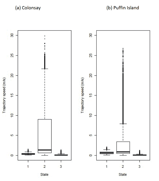
3.5.4 Effects of wind speed on step length (speed)

Wind speed was included in the best-fitting model for Puffin Island, the Isle of May, and Colonsay incorporating TDR dive data (Appendices AD and AE). Step lengths specific to behavioural state (State 1 floating, State 2 transit/commute, State 3 foraging) were plotted in relation to wind speed for models without TDR data and models including TDR. From the Puffin Island model, increasing step lengths are observable in relation to wind speed state 1 (β = 0.029), contrasting a marked decrease in relation to State 3 (β = -0.095) (e.g. Figure 3.127). Puffin Island commuting (State 2) step lengths increased only slightly in relation to wind speed(β = 0.002). For all three states derived from the Isle of May model, step length increased with wind speed, State 1 (β = 0.004), State 2 (β = 0.011), and State 3 (β = 0.013).

In relation to the Colonsay model which incorporated TDR dive data, step lengths decreased with increasing wind speed across State 1 (β = -0.014), and State 3 (β = -0.001), and increased in State 2 (β = 0.001).

3.5.5 Transition effects between states in relation to covariates

AIC selection indicated the best-fitting model for Colonsay contained the covariates (hour + colony distance), Puffin Island and the Isle of May contained all the covariates (hour+ Julian date+ colony distance + wind speed), the model corresponding to Fowlsheugh contained (hour + colony distance) (Appendix AF). Model selection indicated the best-fitting model incorporating TDR dive data for Colonsay contained wind speed as the sole covariate, the best-fitting model corresponding to Fowlsheugh included (hour + colony distance) (Appendix AF), thus being more similar than Colonsay to the standard HMM model for Fowsheugh. Differences between standard HMMs and those further models including TDR data are hard to compare reliably given differences in sample size, but may indicate model sensitivity at Colonsay, individual variation in responses to covariates, and findings could be expected to be more similar for Fowlsheugh than Colonsay given the subset of data is based on one year, thus removing any potential annual biases in representivity.

Birds from Colonsay and the Isle of May exhibited clear relationships with colony distance and transitions between states (Figure 24; Appendix AD), potentially related to distinct foraging locations where birds will consistently transition to a foraging state. However, no definitive relationship was present in relation to Puffin Island, and only a weak relationship was shown for birds from Fowlsheugh. Models incorporating TDR dive data, displayed that birds from Fowlsheugh that decreased commuting and increased floating at greater distances from the colony (Appendix AD).

Julian date appears to influence the extent of commuting and floating at Puffin Island over the course of the tracking period with a peak in floating exhibited at Julian day 170 (Figure 25; Appendix AD). While this may be due environmental effects on behaviour related to season, it should be noted that individuals were not tracked continuously across this period (max = 77.93 hours, Puffin Island max = 79.85 hours, Fowlsheugh). These relatively short tracking periods are potentially subject to breeding stage and individualistic foraging behaviour. Compared with Puffin Island, Fowlsheugh and the Isle of May showed no discernible pattern of influence between Julian date and stationary state probabilities.

Hour of the day produces less defined relationships between behavioural state transitions in Guillemot (Appendix AD) than exhibited by Razorbills. Though, a degree of reduced floating coinciding with increased commuting and foraging is discernible during daylight hours (09:00-15:00) at all colonies. When TDR dive data is incorporated within the model, the relationship of behavioural state with time of day still exhibits a similar pattern (Appendix AD).

Wind speed remained a covariate in the best-fitting model for Puffin Island and the Isle of May (Appendix AF). However, the transition probabilities and stationary state probabilities are unaffected by wind speed at both colonies (Appendix AD). Foraging was largely unaffected by increasing wind speeds, however, floating increased and commuting decreased at standardised values > 2.

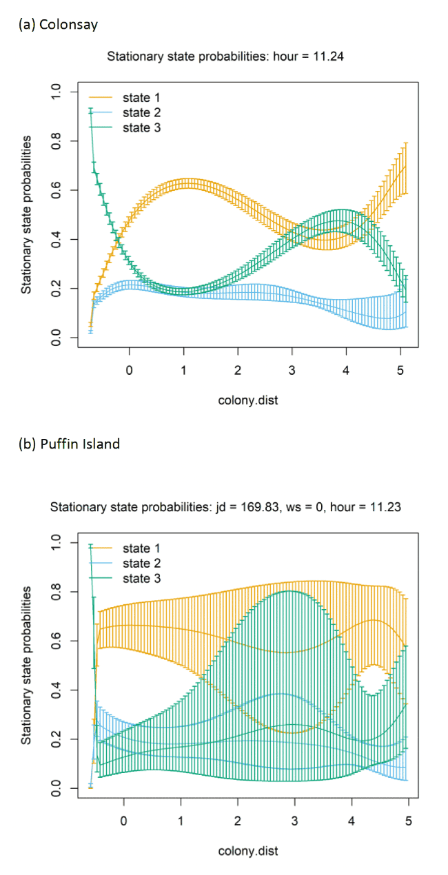
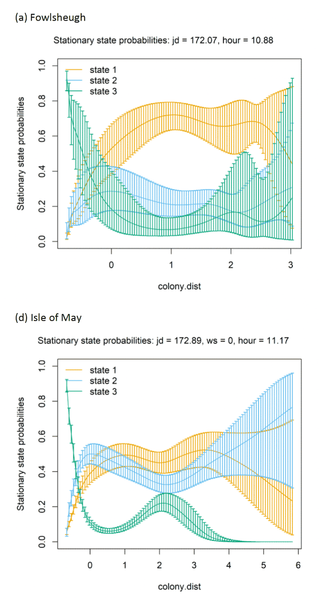
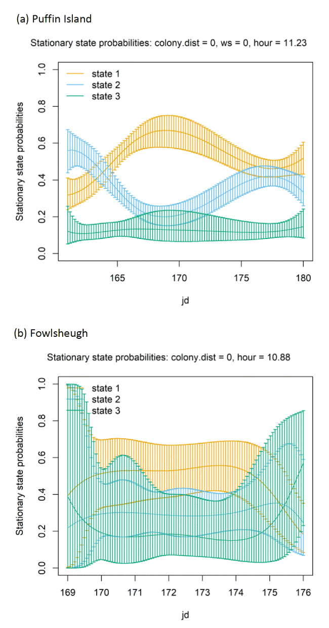
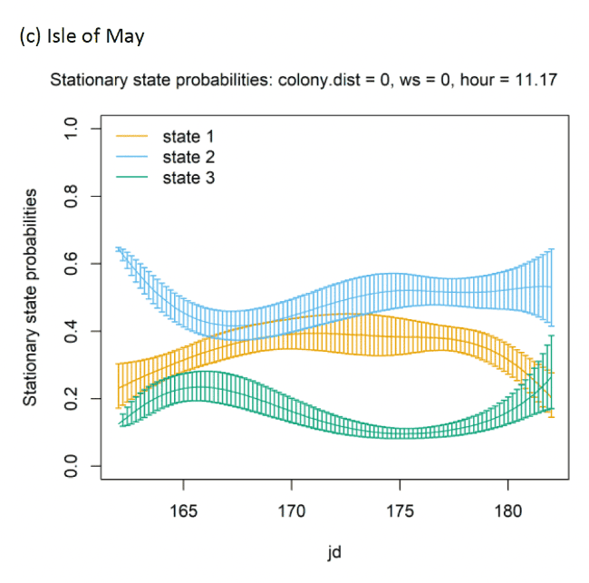
3.5.6 Time in states

The range of duration of data per bird and the proportion of time spent in different states are shown in Table 35. As birds with fewer data had less time to demonstrate their overall time spent in different states, we used information from birds with more than ten hours of data, to exclude any very small tracking durations that could otherwise skew patterns observed. Across all the colonies State 3 (foraging) held the greatest proportion of time, followed by State 1 (floating). State 2 (transit/commuting) held the lowest proportion of time, potentially related to the energetic demands of remaining within that state.

In comparison to non-TDR models, the mean proportion of a State 3 (foraging) is reduced in the models incorporating diving data (Table 35). State 2 (commuting) increases in proportion compared to non-TDR models, potentially as it is encompassing GPS fixes previously regarded as foraging.

Table 35: For Guillemots, estimated time spent in states for each colony for birds at each colony across years; note occasionally initial movement models could not be fitted due to a lack of data available for some individuals, hence the effective sample size feeding into assessments is provided in brackets

		Duration of tracking				Proportion time spent per state
Colony	No. birds total (modelled)	Year	No. birds > 10 hrs tracking data	Duration (hrs) mean ± SD per bird	Tracking data range (hrs)	1 floating mean ± SD	2 commuting mean ± SD	3 foraging / searching mean ± SD
Colonsay	77 (77)	2010 to 2014	76	52.99 ± 23.93	6.20 – 133.29	0.30 ± 0.12	0.17 ± 0.07	0.53 ± 0.13
Puffin Island	40 (27)	2012 to 2013, 2015	25	51.36 ± 13.78	5.76 – 77.93	0.39 ± 0.14	0.16 ± 0.05	0.45 ± 0.14
Fowlsheugh	11 (11)	2012	11	36.07 ± 17.15	17.75 – 79.85	0.32 ± 0.09	0.14 ± 0.04	0.53 ± 0.11
Isle of May	51 (51)	2012 – 2014	51	35.86 ± 16.03	14.37 – 118.71	0.24 ± 0.11	0.14 ± 0.06	0.61 ± 0.13
+ TDR data
Colonsay	29	2011 – 2014	28	51.46 ± 17.61	6.2 – 88.53	0.31 ± 0.12	0.64 ± 0.12	0.05 ± 0.03
Fowlsheugh	7	2012	7	31.35 ± 8.25	21.40 – 42.94	0.32 ± 0.09	0.65 ± 0.09	0.03 ± 0.01

3.5.7 Utilisation distributions

Figures depicting utilization distributions for each colony are shown in Appendix AH. Depending on the colony, there was a smaller amount of data from the very highest wind speeds (greater than 8 m/s) – see also section above comparing use and availability for wind speed distributions.

Where sample sizes of number of fixes and birds used to compute utilisation distributions is low, here taken as less than 100 fixes and less than five birds for the lowest amounts of data (see Appendix AA and methods), then confidence in the overlap result is considered low, and is here indicated as requiring a high degree of caution in interpretation of results. Also highlighted is the proportion of fixes available per split of data, with proportions of less than 5% of the total for the state also flagged up as requiring caution.

Low sample sizes were an issue for guillemots at some colonies. Fowlsheugh in particular did not have enough data for reliable comparisons across many categorisations of the data, in particular for the night-high wind data split, with only one bird providing data, and in once case giving only 13 fixes (for the foraging/searching state) thus being too low for use. For the day-high category at Fowsheugh, likewise only three birds provided data often with less than 100 fixes. For Puffin Island too, for guillemots the nigh-high category for commuting and foraging was based on only one bird with a very small number of fixes. For all colonies except the Isle of May, the number of fixes in the night-high category were less than 5% of the total data available. The Isle of May had higher sample sizes of birds and fixes in each category thus being sufficient for comparison of distribution overlaps.

3.5.8 Overlap indices

Overlaps between states in different wind conditions and times of the day are visualized in Appendix AI, and summarised in Table 36 and Table 37

For Colonsay, Guillemot overlaps between 95% KDEs (representing total area use) were all moderate to very high (BA ≥ 0.4). The highest affinities consistently exhibited across states 1, 2, and 3 were between day high and low wind speed conditions. Day-low vs night high display a degree of moderate affinity (> 0.4) across all states, though affinity is weakest in State 1, further reflected in a low BA index for core area use, as given by the 50% KDE (BA = 0.37). State 3 affinities are consistently high between all conditions. The high affinities between conditions, within all states, is reflective is of the exhibited by Colonsay Razorbills, this is potentially attributed to foraging sympatry.

Puffin Island affinities were consistently high (BA > 0.8) between both day/night low wind conditions across all three states. High vs low wind speeds during the day display affinities > 0.5 between State 2 and 3, with comparatively lower values than Colonsay. However, similar to Colonsay, the overlap affinity between night and day low wind speeds for State 3 is the highest for Puffin Island. As with Colonsay and Puffin Island, day/night low wind speeds are consistently moderate to high in affinity across all three states for Fowlsheugh. Similar to Colonsay, Fowlsheugh produces very high affinities (BA > 0.8) within State 3 between comparisons of conditions. For the Isle of May, BA indices were generally moderate to very high for 95% KDEs, but for 50% KDE overlaps were highly variable across states spanning all ranges of BA indices (very low to very high). Very high overlaps in both 95% and 50% KDEs were seen for State 3 (foraging/searching) across all conditions.

Some overlaps for guillemots showed BA indices of zero, indicating no overlaps – this was apparent for the 50% KDE for Puffin Island and was evident for all states for the comparison of day-low versus night-high conditions, and was also true for the 95% KDE for the same pair-wise comparison for the state of foraging/searching, with further very low overlaps for the other states. Although we caution sample sizes were low in these tests with fewest data available for night-high categorization of the data, this nonetheless indicates differences in area use for Puffin island in particular. However, these patterns were not ubiquitous across other colones – at the Isle of May, for example, 50% KDE overlaps between day-low and night-high were classed as high or very high, being over 0.6 for the states of commuting and foraging/searching.

Overlaps between 95% KDEs for TDR incorporating models for Colonsay and Fowlsheugh, as with the non-TDR models, produce high affinities between day/night low wind speed conditions for State 1, 2. However, in contrast TDR and non-TDR models, day/night low wind speed affinities in relation to State 3 are greatly reduced (Colonsay, BA = 0.51; Fowlsheugh, BA = 0.16). Both TDR incorporating models for Colonsay and Fowlsheugh produce much lower overlap affinities within State 3 than their TDR incorporating counterparts. This may be due in part dive data providing a stringent parameter to the allocation State 3. The highest affinities (BA > 8) are, therefore, displayed in State 2 of TDR models for Colonsay and Fowlsheugh.

Table 36: For Guillemots, overlap indices for combinations of KDEs assessing similarity in 50% and 95% KDEs for different levels of day and night, and high/low wind and states 1, 2 and 3 (floating, commuting and foraging/searching); for example the top row takes the 95% KDEs for daytime low wind conditions for each State 1, 2 and 3, and computes Bhattacharyya's Affinity index for those three distributions, taking a mean and standard deviation, omitting the diagonal of the matrix that compares each the distribution to itself; note for the comparison of day and night (across wind conditions) for specific states, this results in a simple 2 x 2 matrix and thus, only one comparison value that cannot therefore have a standard deviation; red highlight shows where confidence in overlap assessment is lowest due to low sample sizes (see methods and Appendix AA).

(a) Colonsay

state		day.high	day.low	night.high
1	day.low	0.54 (0.4)
1	night.high	0.41 (0.25)	0.42 (0.37)
1	night.low	0.52 (0.34)	0.75 (0.53)	0.4 (0.31)
2	day.low	0.78 (0.72)
2	night.high	0.58 (0.61)	0.57 (0.62)
2	night.low	0.72 (0.66)	0.81 (0.7)	0.48 (0.53)
3	day.low	0.91 (0.97)
3	night.high	0.89 (0.93)	0.88 (0.95)
3	night.low	0.87 (0.97)	0.91 (0.95)	0.84 (0.94)

(b) Puffin Island

state		day.high	day.low	night.high
1	day.low	0.33 (0)
1	night.high	0.59 (0.16)	0.3 (0)
1	night.low	0.24 (0)	0.81 (0.6)	0.25 (0)
2	day.low	0.55 (0.48)
2	night.high	0.18 (0)	0.15 (0)
2	night.low	0.43 (0.37)	0.84 (0.75)	0.26 (0.22)
3	day.low	0.87 (0.9)
3	night.high	0.02 (0)	0 (0)
3	night.low	0.75 (0.95)	0.88 (0.86)	0.06 (0)

(c) Fowlsheugh

state		day.high	day.low	night.high
1	day.low	0.25 (0.1)
1	night.high	0.14 (0)	0.25 (0.13)
1	night.low	0.24 (0.09)	0.52 (0.45)	0.15 (0)
2	day.low	0.47 (0.33)
2	night.high	0.15 (0.02)	0.36 (0.07)
2	night.low	0.31 (0.23)	0.68 (0.81)	0.29 (0.08)
3	day.low	0.82 (0.81)
3	night.high	0.85 (0.86)	0.91 (0.84)
3	night.low	0.84 (0.83)	0.96 (0.96)	0.94 (0.86)

(d) Isle of May

state		day.high	day.low	night.high
1	day.low	0.46 (0.32)
1	night.high	0.52 (0.36)	0.42 (0.26)
1	night.low	0.32 (0.17)	0.62 (0.46)	0.32 (0.17)
2	day.low	0.71 (0.66)
2	night.high	0.6 (0.63)	0.61 (0.75)
2	night.low	0.55 (0.57)	0.72 (0.73)	0.57 (0.69)
3	day.low	0.94 (0.91)
3	night.high	0.91 (0.95)	0.9 (0.86)
3	night.low	0.88 (0.87)	0.92 (0.91)	0.84 (0.86)

Table 37: For Guillemots, overlap indices for combinations of KDEs, using a subset of birds with GPS+TDR data (from HMMs including the additional channel of dive for refined state assignment); for details of overlap tables see Table 36 above.

(a) Colonsay

state		day.high	day.low	night.high
1	day.low	0.47 (0.4)
1	night.high	0.42 (0.21)	0.29 (0.27)
1	night.low	0.39 (0.24)	0.61 (0.41)	0.22 (0.21)
2	day.low	0.84 (0.92)
2	night.high	0.8 (0.85)	0.82 (0.91)
2	night.low	0.8 (0.96)	0.89 (0.95)	0.79 (0.88)
3	day.low	0.36 (0.16)
3	night.high	0.38 (0.3)	0.16 (0.06)
3	night.low	0.29 (0.08)	0.51 (0.21)	0.05 (0)

(b) Fowlsheugh

state		day.high	day.low	night.high
1	day.low	0.08 (0)
1	night.high	0.1 (0)	0.23 (0.17)
1	night.low	0.02 (0)	0.51 (0.46)	0.1 (0)
2	day.low	0.04 (0)
2	night.high	0.08 (0)	0.1 (0)
2	night.low	0 (0)	0.9 (0.91)	0.01 (0)
3	day.low	0.07 (0)
3	night.high	0.15 (0)	0.13 (0)
3	night.low	0 (0)	0.16 (0.06)	0 (0)

3.6 Species summary

All species for the State 1 behaviour (floating) had a generally very-low or low-moderate overlap of day-low conditions of 50% KDEs with the night-high wind conditions; overlaps with this opposing condition for floating were lowest in all the three pair-wise comparisons that included day-low conditions and across all states. The greatest general overlap across species was seen for the day-low versus day-high comparison for commuting and foraging/searching, with frequent affinities across species being typically high or very high. Greatest general disparity was between day-low and night-high conditions, although note, that in many cases, sample size was an issue for these comparisons.

Between species, the auks (and also Kittiwakes) showed generally lower overlaps than Lesser Black-backed Gulls and Gannets commuting, although patterns were quite varied. Conversely, the auks (using non-TDR data) showed greater overlaps for the foraging/searching state, particularly for the day-low vs night-high comparison, than other species, although again with variation – note Puffin Island was an exception to this pattern.

Overall, although there was much variation, the average BA index (see: 2.5 Overlap analyses) across all pair-wise comparisons in Table 38 (GPS + TDR in Table 39) below, was 0.65 ± 0.20 for the 95% KDE and 0.51 ± 0.28 for the 50% KDE, indicating a highly generalised 'high' degree of spatial overlap in distributions across conditions, states, species and colonies, and a moderate overlap for the 50% KDE.

Table 38: Comparison of Bhattacharrya's Affinity indices between day-low wind scenarios, representative of suitable survey conditions, with other conditions (day-high, night-low and night-high), split by behavioural state, arranged by species and colony, coloured by BA index values very low – very high five-tier categorisation (see section 2.5); cells highlighted with asterisk indicates lowest confidence in overlaps due to lowest sample sizes (see methods and Appendix AA). LBBG = Lesser Black-baked Gull.

			95% KDE			50% KDE
State	Species	Colony	day-high	night-high	night-low	day-high	night-high	night-low
1	Gannet	Alderney	0.61	0.55	0.75	0.34	0.21	0.58
		Bass Rock	0.52	0.40	0.69	0.19	0.15	0.49
	LBBG	Orford Ness	0.47*	0.40*	0.60	0.45*	0.14*	0.37
		Skokholm	0.77	0.56	0.72	0.46	0.28	0.39
		Walney	0.37*	0.37	0.59	0.06*	0.08	0.29
	Kittiwake	Bempton	0.47	0.34	0.63	0.28	0.15	0.45
		Colonsay	0.61	0.44	0.66	0.67	0.17	0.58
		Isle of May	0.46*	0.34*	0.52	0.21*	0.28*	0.29
		Orkney	0.74	0.47	0.61	0.77	0.07	0.45
	Razorbill	Colonsay	0.77	0.69	0.77	0.55	0.58	0.49
		Isle of May	0.53	0.28*	0.60	0.58	0.04*	0.40
		Puffin Island	0.48	0.40	0.78	0.23	0.15	0.61
	Guillemot	Colonsay	0.54	0.42	0.75	0.40	0.37	0.53
		Fowlsheugh	0.25*	0.25*	0.52	0.10*	0.13*	0.45
		Isle of May	0.46	0.42	0.62	0.32	0.26	0.46
		Puffin Island	0.33	0.30	0.81	0.00	0.00	0.60
2	Gannet	Alderney	0.90	0.58	0.74	0.73	0.26	0.39
		Bass Rock	0.88	0.65	0.87	0.72	0.38	0.80
	LBBG	Orford Ness	0.90	0.63	0.92	0.84	0.33	0.90
		Skokholm	0.90	0.81	0.92	0.85	0.70	0.84
		Walney	0.84	0.68	0.88	0.60	0.42	0.60
	Kittiwake	Bempton	0.80	0.51	0.82	0.58	0.32	0.79
		Colonsay	0.73	0.60	0.83	0.74	0.63	0.72
		Isle of May	0.62	0.43*	0.72	0.56	0.29*	0.65
		Orkney	0.69	0.56	0.72	0.70	0.46	0.68
	Razorbill	Colonsay	0.91	0.67	0.80	0.91	0.50	0.54
		Isle of May	0.79	0.31*	0.70	0.97	0.00*	0.69
		Puffin Island	0.74	0.25	0.57	0.48	0.00	0.15
	Guillemot	Colonsay	0.78	0.57	0.81	0.72	0.62	0.70
		Fowlsheugh	0.47*	0.36*	0.68	0.33*	0.07*	0.81
		Isle of May	0.71	0.61	0.72	0.66	0.75	0.73
		Puffin Island	0.55	0.15*	0.84	0.48	0.00*	0.75
3	Gannet	Alderney	0.75	0.50	0.78	0.60	0.14	0.68
		Bass Rock	0.68	0.46	0.74	0.33	0.15	0.53
	LBBG	Orford Ness	0.71	0.50	0.77	0.59	0.22	0.43
		Skokholm	0.85	0.57	0.80	0.56	0.24	0.35
		Walney	0.72	0.55	0.82	0.50	0.12	0.54
	Kittiwake	Bempton	0.57	0.32	0.75	0.37	0.03	0.68
		Colonsay	0.72	0.54	0.81	0.72	0.40	0.76
		Isle of May	0.59	0.48*	0.71	0.48	0.39*	0.58
		Orkney	0.87	0.82	0.86	0.90	0.93	0.97
	Razorbill	Colonsay	0.96	0.86	0.87	0.96	0.85	0.82
		Isle of May	0.99	0.79*	0.92	0.98	0.79*	0.92
		Puffin Island	0.78	0.06*	0.63	0.87	0.00*	0.52
	Guillemot	Colonsay	0.91	0.88	0.91	0.97	0.95	0.95
		Fowlsheugh	0.82*	0.91*	0.96*	0.81*	0.84*	0.96*
		Isle of May	0.94	0.90	0.92	0.91	0.86	0.91
		Puffin Island	0.87	0.00	0.88	0.90	0.00	0.86

Table 39: Additional overlap summary of the auks using GPS+ TDR HMM classifications, to supplement Table 38; comparison of Bhattacharrya's Affinity indeces between day-low wind scenarios, representative of suitable survey conditions, with other conditions (day-high, night-low and night-high), split by behavioural state, arranged by species and colony, coloured by BA index values very low – very high five-tier categorisation (see section 2.5 in methods)

			95% KDE			50% KDE
State	Species	Colony	day-high	night-high	night-low	day-high	night-high	night-low
1	Razorbill	Colonsay
	Guillemot	Colonsay	0.47	0.29	0.61	0.4	0.27	0.41
		Fowlsheugh	0.08	0.23	0.51	0	0.17	0.46
2	Razorbill	Colonsay
	Guillemot	Colonsay	0.84	0.82	0.89	0.92	0.91	0.95
		Fowlsheugh	0.04	0.1	0.9	0	0	0.91
3	Razorbill	Colonsay
	Guillemot	Colonsay	0.36	0.16*	0.51	0.16	0.06*	0.21
		Fowlsheugh	0.07*	0.13*	0.16*	0*	0*	0*