Improving Our Understanding of Seabird Behaviour at Sea

This project collated tracking data from five seabird species thought to be vulnerable to offshore wind farms. These data were analysed to understand whether seabird distribution data, usually undertaken in daytime, good weather conditions, were representative of behaviour in other conditions.

This document is part of a collection


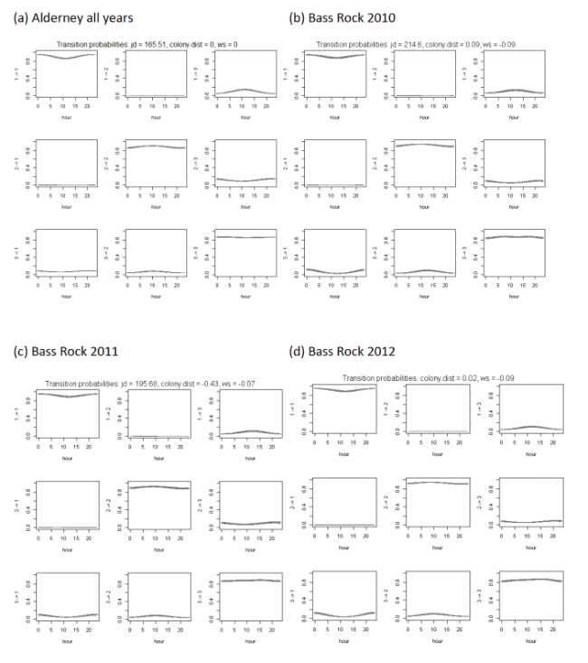
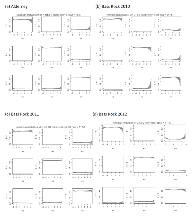
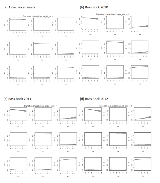
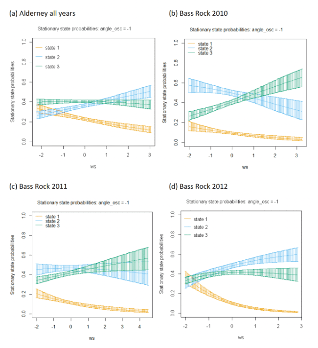
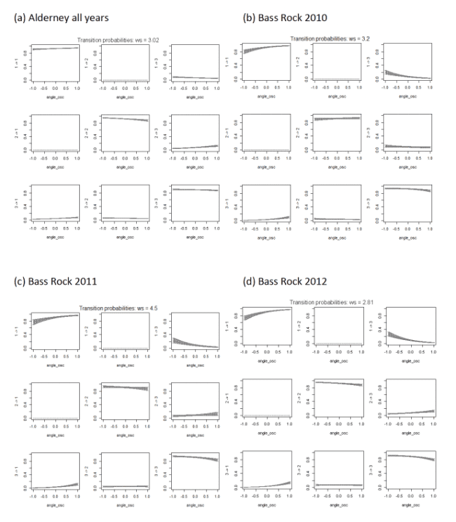
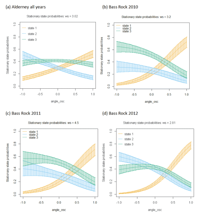
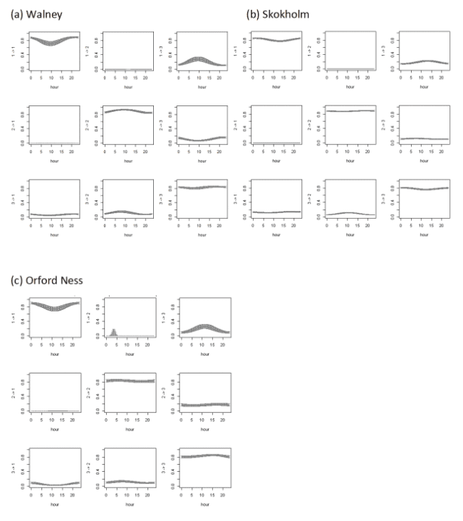
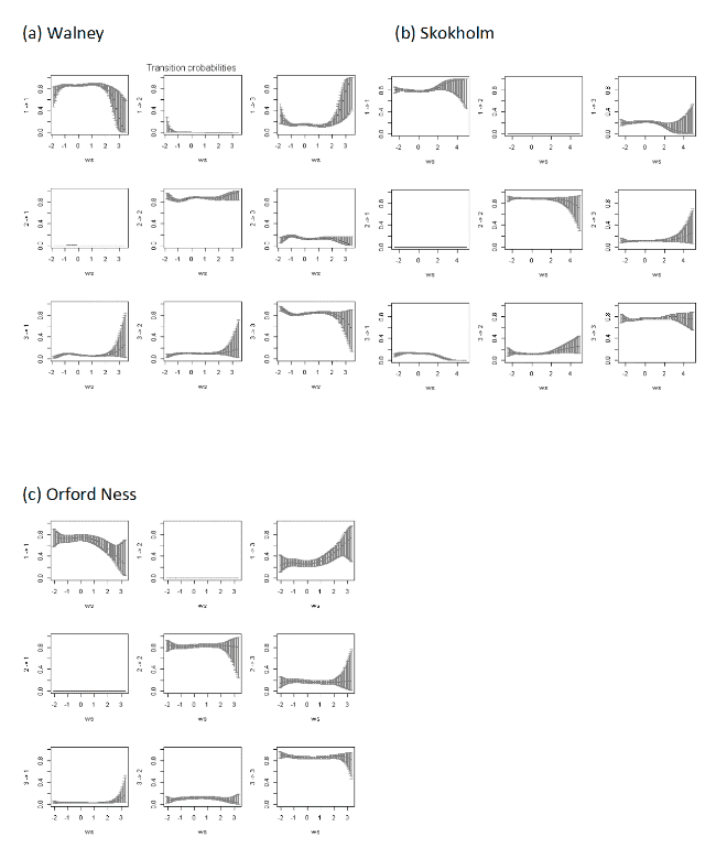
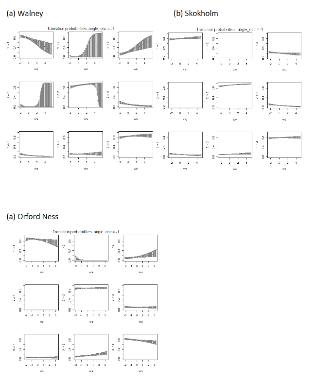
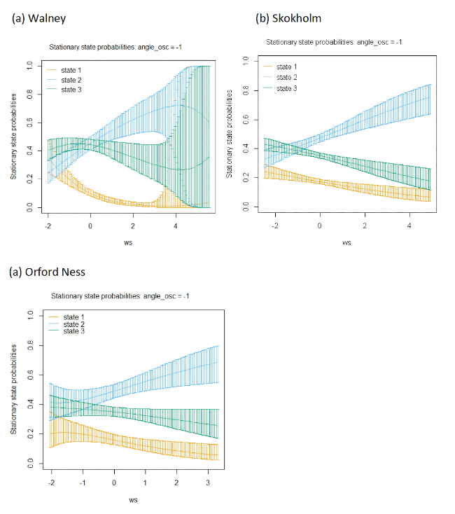
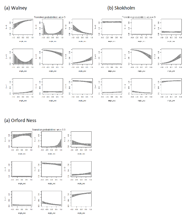
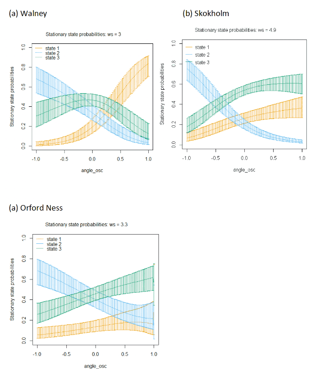
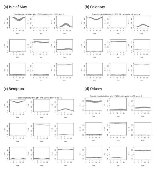
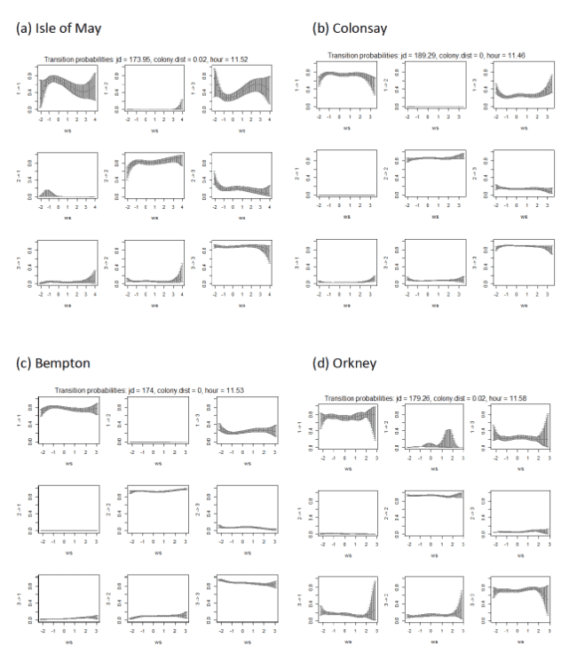
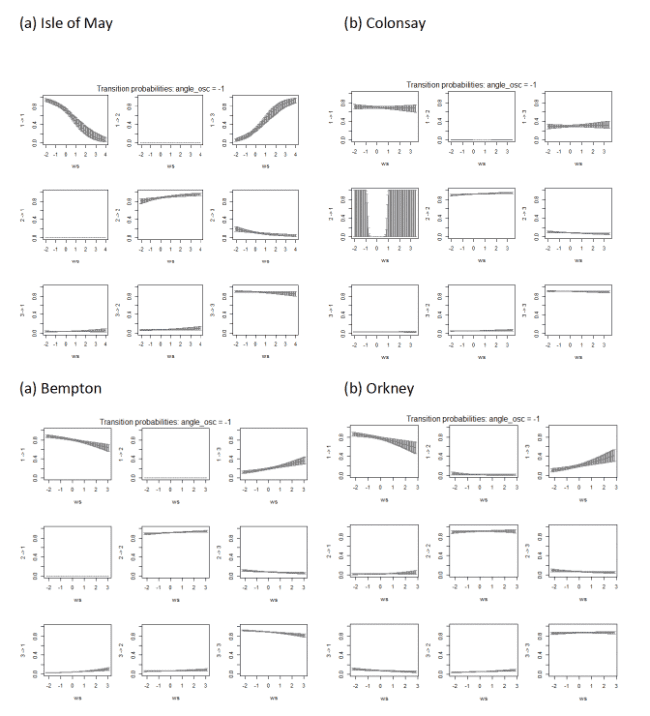
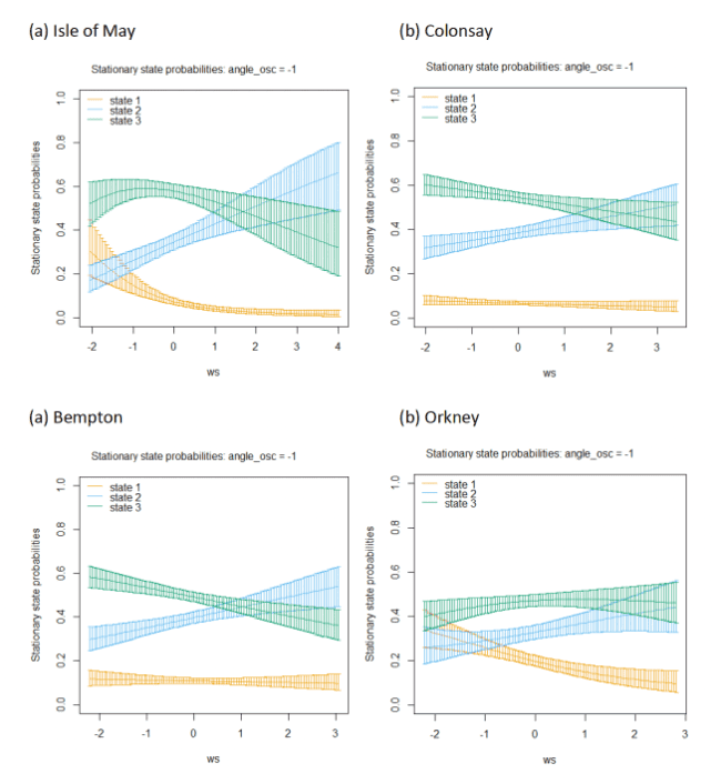
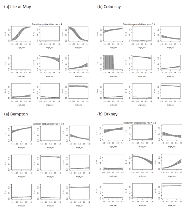
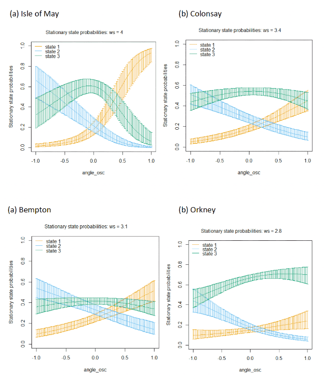
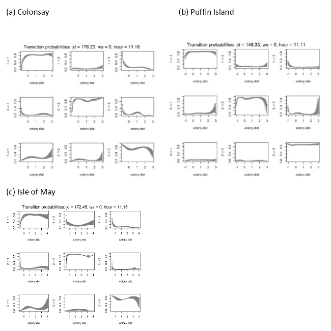
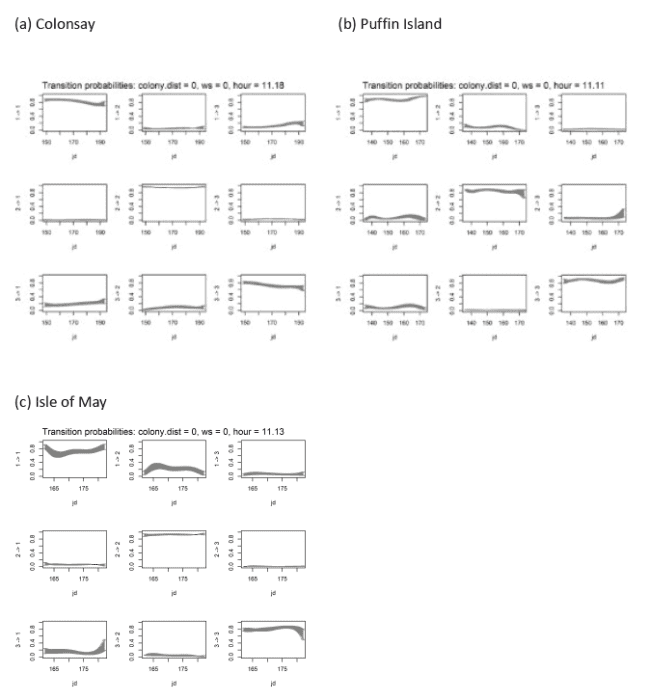
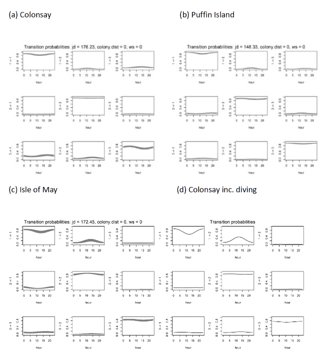
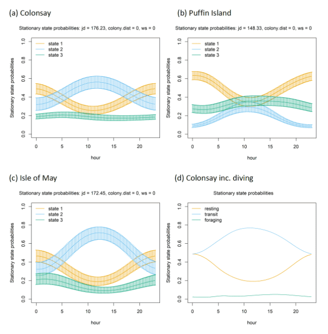
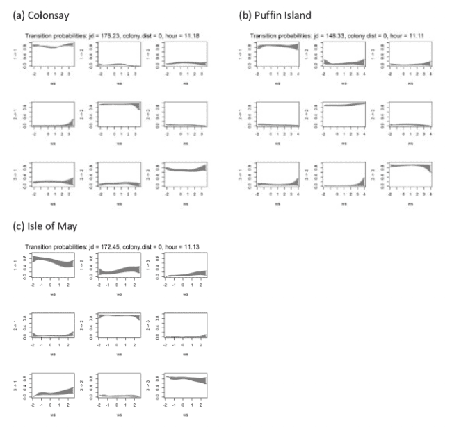
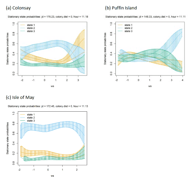
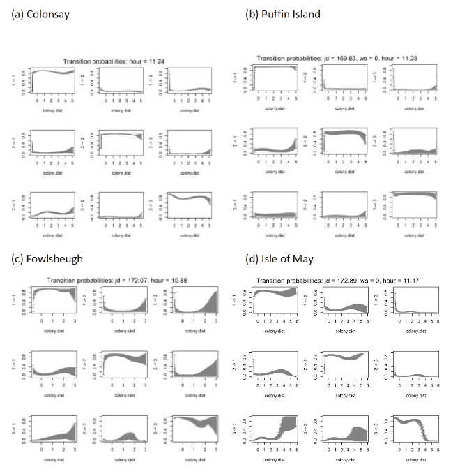
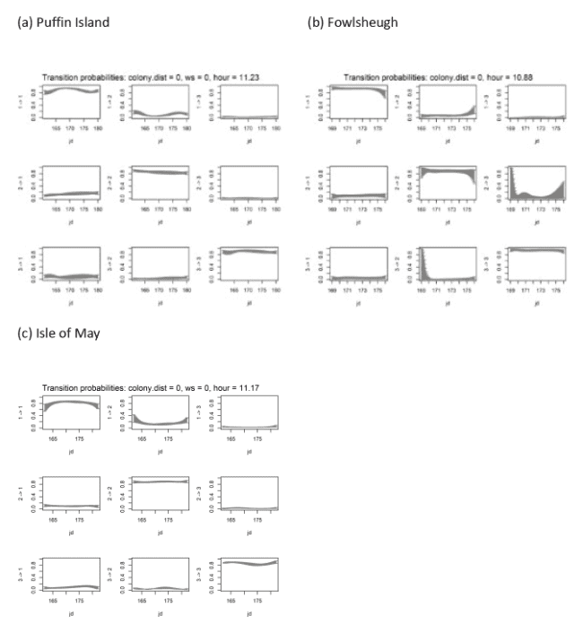
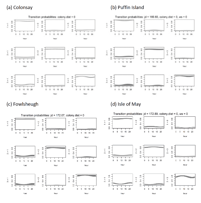
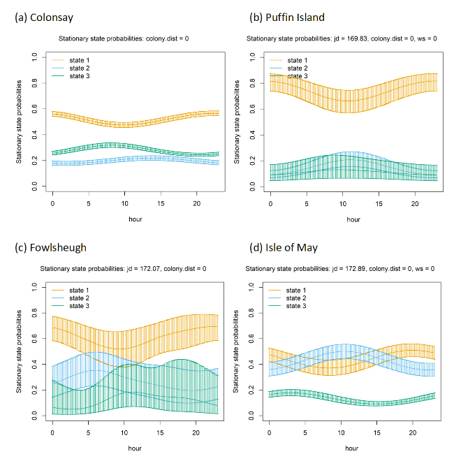
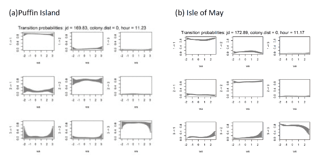
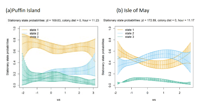
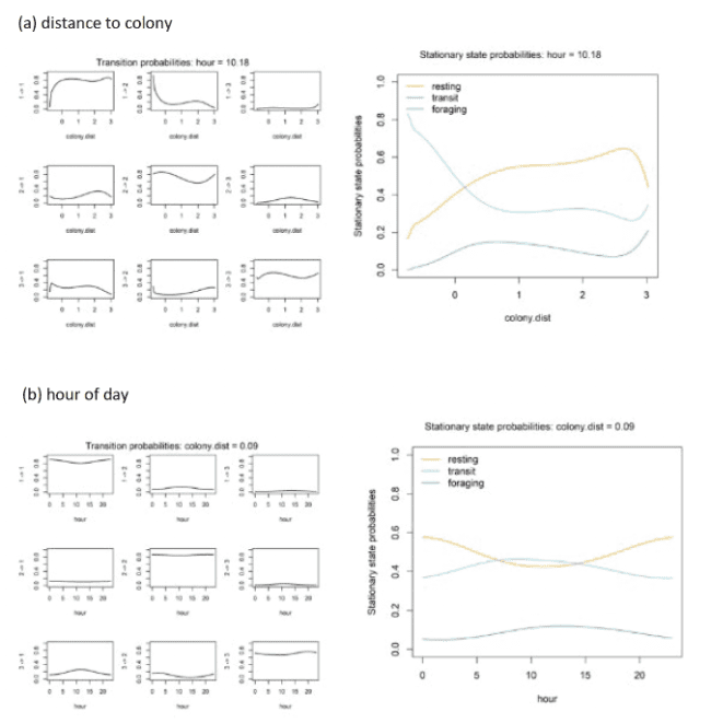
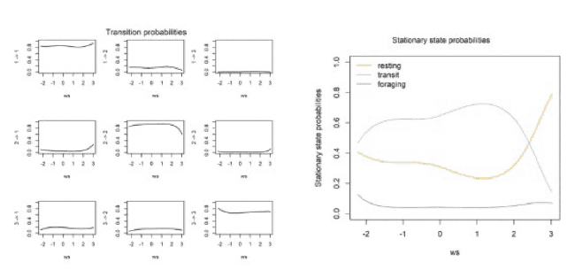
7.4 Appendix AD. Transition effects between states in relation to covariates

Plots are generated for specific covariates at the means of other covariates in the model. The range of wind speeds, as with other covariates, within plots are presented as standardised values. The following corresponding range of real wind speed values is given as follows to aid interpretation:

  • Gannet: Alderney, 0.03 – 14.45 (6.26 ± 2.83) m/s; Bass Rock, 0.03 – 18.02 (5.59 ± 2.76) m/s;
  • Lesser Black-backed Gulls (offshore): Walney, 0.07 m/s – 13.34 (4.69 ± 2.49) m/s; Skokholm, 0.04 m/s – 16.67 (5.31 ± 2.22) m/s; Orford Ness 0.04 m/s – 12.46 (4.99 ± 2.56) m/s;,
  • Kittiwake: Isle of May, 0.18 m/s – 13.19 (4.60 ± 2.14) m/s; Colonsay, 0.07 – 13.94 (5.24 ± 2.55) m/s; Bempton Cliffs, 0.03 – 12.26 (5.15 ± 2.32) m/s; Orkney, 0.05 – 12.63 (5.58 ± 2.50) m/s;
  • Razorbill: Colonsay, 0.03 – 14.26 m/s; Puffin Island, 0.05 – 14.81 m/s (4.77 ± 2.77); Isle of May, 0.17 – 10.29 (4.53 ± 2.51) m/s;
  • Guillemot: Puffin Island, 0.25 m/s – 9.36 (3.86 ± 2.11) m/s, Isle of May, 0.20 – 11.8 (4.96 ± 2.08) m/s, Colonsay, 0.06 m/s – 11.26 (4.68 ± 2.42) m/s; Fowlseugh 0.60 m/s – 12.91 (5.30 ± 2.29) m/s.

7.4.1 Northern Gannet

Figure A40: For Gannet, transition probabilities and stationary state probabilities for the variable of cosinor(hour of day).
described in body of report
Figure A41: For Gannet, transition probabilities for the variable of bSpline(wind speed), fitted as a standardised variable.
described in body of report
Figure A42: For Gannet, transition plots for wind speed in interation with angular_osc (travel direction alignment to wind direction, -1 = direct headwind, +1 = direct tailwind), here plotted for a full headwind (-1) over varying wind speed, showing effects on transition between states.
described in body of report
Figure A43: For Gannet, stationary state probability plots for wind speed in interation with angular_osc (travel direction alignment to wind direction, -1 = direct headwind, +1 = direct tailwind), here plotted for a full headwind (-1) over varying wind speed, for states 1, 2 and 3 (floating, commuting and foraging/searching).
described in body of report
Figure A44: For Gannet, transition plots for wind speed in interation with angular_osc (travel direction alignment to wind direction, -1 = direct headwind, +1 = direct tailwind), plotted for a varying values of angular_osc for strongest wind speeds.
described in body of report
Figure A45: Stationary state probability plots for wind speed in interation with angular_osc (travel direction alignment to wind direction, -1 = direct headwind, +1 = direct tailwind), plotted for a varying values of angular_osc for strongest wind speeds per colony for states 1, 2 and 3 (floating, commuting and foraging/searching).
described in body of report

7.4.2 Lesser Black-backed Gull

Figure A46: For Lesser Black-backed Gull, transition probabilities for the variable of cosinor(hour of day).
described in body of report
Figure A47: For Lesser Black-backed Gull, transition probabilities for the variable of bSpline(wind speed), fitted as a standardised variable.
described in body of report
Figure A48: For Lesser Black-backed Gull, transition probabilities over time t and t+1 depicting the interaction of wind speed with angular_osc (travel direction alignment to wind direction, -1 = direct headwind, +1 = direct tailwind), here plotted for varying wind speeds (standardised variable range per colony), for headwinds (angular_osc = -1).
described in body of report
Figure A49: For Lesser Black-backed Gull, stationary state probabilities (i.e. likelihood of point being classified as a particular state) depicting wind speed in interation with angular_osc (travel direction alignment to wind direction, -1 = direct headwind, +1 = direct tailwind), here plotted for a full headwind (-1) over varying wind speed, showing effects on transition between states; see above for details on the standardised variable of wind speed and it's equivalent true valules of wind speed for each colony.
described in body of report
Figure A50: For Lesser Black-backed Gull, transition probabilities between states over time t and t+1 depicting the interaction of wind speed with angular_osc (travel direction alignment to wind direction, -1 = direct headwind, +1 = direct tailwind), here plotted for a varying values of angular_osc for strongest wind speeds per colony (3.0, 4.9 and 3.3 for Walney, Skokholm and Orford Ness, respectively), equating to ca. 11.4 m/s, 16.0 m/s and 12.9 m/s for Walney, Skokholm and Orford Ness; note large errors at the tail end of the Walney model up to max wind (17.4 m/s) produced the same patterns but with low confidence in the trends.
described in body of report
Figure A51: For Lesser Black-backed Gull, stationary state probabilities depicting the interaction of wind speed with angular_osc (travel direction alignment to wind direction, -1 = direct headwind, +1 = direct tailwind), here plotted for a varying values of angular_osc for strongest wind speeds per colony (3.0, 4.9 and 3.3 for Walney, Skokholm and Orford Ness, respectively), equating to ca. 11.4 m/s, 16.0 m/s and 12.9 m/s for Walney, Skokholm and Orford Ness; note large errors at the tail end of the Walney model up to max wind (17.4 m/s) produced the same patterns but with low confidence in the trends.
described in body of report

7.4.3 Black-legged Kittiwake

Figure A52: For Kittiwake, transition probabilities for the variable of cosinor (hour of day).
described in body of report
Figure A53: For Kittiwake, transition probabilities for the variable of bSpline(wind speed), fitted as a standardised variable.
described in body of report
Figure A54: For Kittiwake, transition probabilities between states over time t and t+1 depicting the interaction of wind speed with angular_osc (travel direction alignment to wind direction, -1 = direct headwind, +1 = direct tailwind), here plotted for varying wind speeds (standardised variable range per colony), for headwinds (angular_osc = -1).
described in body of report
Figure A55: For Kittiwake, stationary state probabilities (i.e. likelihood of point being classified as a particular state) depicting the interaction of wind speed with angular_osc (travel direction alignment to wind direction, -1 = direct headwind, +1 = direct tailwind), here plotted for a varying values of wind speed for for tailwinds (angle_osc = +1).
described in body of report
Figure A56: For Kittiwake, transition probabilities between states over time t and t+1 depicting the interaction of wind speed with angular_osc (travel direction alignment to wind direction, -1 = direct headwind, +1 = direct tailwind), here plotted for a varying values of angular_osc for strongest wind speeds per colony.
described in body of report
Figure A57: For Kittiwake, stationary state probabilities depicting the interaction of wind speed with angular_osc (travel direction alignment to wind direction, -1 = direct headwind, +1 = direct tailwind), here plotted for a varying values of angular_osc for strongest wind speeds per colony.
described in body of report

7.4.4 Razorbill

Figure A58: For Razorbill, transition probabilities for the variable of distance to colony, fitted as a standardised variable.
described in body of report
Figure A59: For Razorbill, transition probabilities for the variable of Julian date at (a) Colonsay,(b) Puffin Island and (c) Isle of May.
described in body of report
Figure A60: For Razorbill, transition probabilities for the variable of cosinor(hour of day) at (a) Colonsay,(b) Puffin Island and (c) Isle of May (d) Colonsay + TDR.
described in body of report
Figure A61: For Razorbill, stationary state probabilities for the variable of cosinor(hour of day) at (a) Colonsay, (b) Puffin Island, and (c) the Isle of May,(d) Colonsay + TDR.
described in body of report
Figure A62: For Razorbill, transition probabilities for the variable of bSpline(wind speed), fitted as a standardised variable
described in body of report
Figure A63: For Razorbill, stationary state probabilities for the variable of bSpline(wind speed), fitted as a standardised variable.
described in body of report

7.4.5 Common Guillemot

Figure A64: For Guillemot, transition probabilities for the variable of distance to colony, fitted as a standardised variable.
described in body of report
Figure A65: For Guillemot, transition probabilities for the variable of Julian date.
described in body of report
Figure A66: For Guillemot, transition probabilities for the variable of cosinor(hour of day).
described in body of report
Figure A67: For Guillemot, stationary state probabilities for the variable of cosinor(hour of day).
described in body of report
Figure A68: For Guillemot, transition probabilities for the variable of bSpline(wind speed), fitted as a standardised variable.
described in body of report
Figure A69: For Guillemot, stationary state probabilities for the variable of bSpline(wind speed), fitted as a standardised variable
described in body of report
Figure A70: For Guillemot, transition and stationary state probabilities at Fowlsheugh from models incorporating TDR dive data for the variables of distance to colony and cosinor(hour of day).
described in body of report
Figure A71: For Guillemot, transition and stationary state probabilities at Colonsay from models incorporating TDR dive data for the variable of bSpline(wind speed), fitted as a standardised variable.
described in body of report

Contact

Email: ScotMER@gov.scot

Back to top