Improving Our Understanding of Seabird Behaviour at Sea

2 Methods

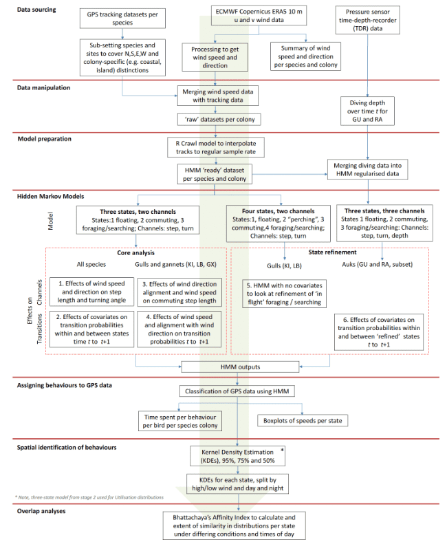
The workflow within this project is summarised in a schematic (Figure 1), which highlights the acquisition and application of raw datasets included within the study, their preparation and manipulation, leading further through the stages of behavioural and spatial analyses. We highlight flows of information through each stage, with key final outputs and summaries of information also highlighted.

2.1 Data sourcing

2.1.1 Study species

We considered a total of nine species of UK seabird for potential inclusion within this project: Northern Gannet, hereafter 'Gannet' (Morus bassanus), European Shag (Phalacrocorax aristotelis), Lesser Black-backed Gull (Larus fuscus), Herring Gull (Larus argentatus), Great Black-backed Gull (Larus marinus), Black-legged Kittiwake, herafter 'Kittiwake' (Rissa Trydactyla), Common Guillemot, hereafter 'Guillemot' (Uria aalge), Razorbill (Alca torda) and Atlantic Puffin (Fratercula arctica). However, these species were reduced to a subset of six species (Gannet, Lesser Black-backed Gull, Herring Gull, Kittiwake, Guillemot and Razorbill, Table 1) that were identified as priority species based on perceived importance within impact assessments and policy relevance. Data for these six species were then acquired and for each species we selected key sites from a wider available tracking dataset to, where possible, represent a mix of colonies from north to south and east to west per species, as well as coastal and island colonies for gulls. For Herring Gull, however, the amount of data collected in the offshore environment was very small across datasets, and so was not modelled as part of this study, reducing the number of species presented to five (Table 1).

2.1.2 GPS data

GPS data were acquired from various data sources. Tracking data for guillemots, Razorbills, Kittiwakes and herring gulls were obtained from the RSPB and CEH through the FAME-STAR consortium (Wakefield et al. 2017). Gannet data for Bass Rock were obtained from the University of Leeds and for Alderney from the University of Liverpool (Warwick-Evans et al. 2016; Soanes et al. (2012). Tracking data for Lesser Black-backed Gulls and Herring gulls were obtained through the BTO.

Table 1: Breakdown of the species and sites covered in this project, with information on numbers of birds and years available for each site, east/west, north/south location of the site, whether and island of mainland colony and the colony size at each site for each species. LBBG = Lesser Black-backed Gull.

Species	Colony	N Birds	N Years	East/ West	North/ South	Island/ Mainland	Colony size
Gannet	Alderney	61	4	West	South	Island	5765
Gannet	Bass Rock	133	4	East	Central	Island	75259
LBBG	Orford Ness	25	3	East	South	Mainland	640
LBBG	Walney	54	4	West	Central	Mainland	4987
LBBG	Skokholm	25	2	West	South	Island	1486
Kittiwake	Isle of May	50	3	East	Central	Island	3433
Kittiwake	Orkney	86	5	Central	North	Mainland	~
Kittiwake	Colonsay	84	5	West	North	Island	~
Kittiwake	Bempton Cliffs	104	6	East	Central	Mainland	37617
Guillemot	Isle of May	48	3	East	Central	Island	21598
Guillemot	Colonsay	77	5	West	North	Island	~
Guillemot	Puffin Island	40	5	West	South	Island	3627
Guillemot	Fowlsheugh	11	1	East	North	Mainland	55507
Razorbill	Puffin Island	58	5	West	South	Island	592
Razorbill	Isle of May	28	3	East	Central	Island	4590
Razorbill	Colonsay	42	5	West	North	Island	~

2.1.3 TDR data

Time-Depth Recorders (TDRs) were attached to 29 Guillemots from Colonsay and seven Guillemot from Puffin Island and 26 Razorbills from Colonsay; these deployments were in addition to GPS tags attached to birds (dual deployment) to identify dive locations. TDR pressure recordings were taken at 1 second intervals and were used in this study to refine classification of foraging behaviour for guillemots and Razorbills.

2.1.4 Covariates: Wind speed, direction and time of day

To test whether behaviour and area use of birds differed under different times of the day and in different wind speeds, we specified additional covariates alongside the prepared GPS data ahead of further use-availability assessments and behavioural modelling. Hour of the day (UTC) and Julian date were extracted from the date-times of GPS fixes. The distance (Rhumb line loxodrome) of GPS points to the breeding colony for the species of interest were also specified for inclusion within behavioural analyses (see below). Wind speed and direction data were obtained through the European Centre for Medium Range Weather Forecasts (ECMWF) 'ERA5' reanalysis model, and the mean 10 m u and v wind components were extracted at hourly temporal resolution and ca. 30 km spatial grid resolution (ECMWF 2019). Grid squares were then matched to the GPS locations for each colony and species, ahead of further analyses.

2.1.5 Summary of wind speed and direction experienced by GPS tracked birds relative to that available over the period of GPS tracking per colony

The wind speeds that birds experience at sea may or may not be a reflection of the conditions available to them, for example if they avoid particular conditions such as times when wind speeds are high by either remaining at the colony or (for generalist species) foraging inland rather than offshore. Further, the period of tracking itself is often restricted to a phase during the breeding season, which may or may not reflect the general conditions in the area for the month of study.

For this assessment the mean and maximum wind speed and mean wind direction that individual birds encountered for each colony and year were summarized as an indication of the conditions birds actually experienced during their periods of tracking. To gain perspective how this 'use' of conditions compared to that 'available' in the area, we also extracted wind speed and direction information from each 30 km Copernicus grid square (matched to the GPS data as above) that GPS tracks of birds overlapped with. This availability assessment was conducted for two temporal scales: (i) the entire months in which tracking at the colony and year had been conducted and (ii) the specific tracking durations of individual birds. This enabled a comparison of conditions birds could have experienced across the entire month (for example should tracking have been conducted across a wider period in the months of tracking), and across individual tracking durations of birds (if birds had used all areas equally, albeit with a caveat that more distant offshore areas naturally may be windier).

To present use-availability assessments in a meaningful way specific to the aims of this project, we quantified the proportional use of wind speeds above that deemed too windy for aerial and boat-based surveys to be carried out. We examined the proportion of grid cells per hour, per day that had mean wind speeds greater than 8 m/s and 10 m/s, representing an equivalency to wind speed thresholds above which planes are unlikely able to survey an area (being equivalent to ca. Beaufort Scale 5) and thus informed proportion of use and availability that may be outside of these survey windows for each species, colony and year. This was examined for (a) the grid cells that birds used on a given date and time, (b) those that could have been used at the two temporal scales described. A lower and upper threshold of this window were also specified – see below – to maximize the GPS data available when carrying out investigations of utilization distributions within high and low wind categories.

Proportional use-availability comparisons data were summarised as histograms and spatial plots, using code adapted from the R:rWind package (Fernández‐López & Schliep 2018). We note, however, that this is not a full resource-selection approach and further statistical assessment would be needed to fully understand how birds interacted with particular conditions.

2.2 Data Manipulation

Wind speed and direction data were extracted from raster Copernicus layers and matched to GPS data using a simple overlap of GPS points over Copernicus grid squares and a point-in-polygon assessment. This manipulation step also informed the patterns of use of particular wind speeds in relation to that available as introduced above. This ensured that for further analyses, each GPS fix then had a geo-referenced wind speed and wind direction value appropriately assigned. Time of day was specified as a continuous (circular) covariate for behavioural modelling – see below – which was automatically available for timestamped GPS data. Further data manipulation was also carried out below in an initial step prior to further behavioural modelling – see Section 2.3 below. Further divisions of data for wind speed and time of day were used for assessment of area use – see Section 2.4 below.

2.3 Behavioural modelling

2.3.1 Interpolation of GPS tracks to obtain regular sampling rates

GPS data, although collected under specified sampling rates in each study (five minutes for gulls), and 100-120 seconds for other species, suffer variations in precision delivering a GPS fix at precise rates, due to issues such as signal retention, time-to-fix, and many other variables. For subsequent behavioural analyses, a requirement is that data are "regular" in date and time, necessitating interpolation to translate GPS points to a regular interval so that step lengths and turning angles can be analysed without bias of time variation. To achieve this, we used R package:crawl to fit continuous-time correlated random walk (CTCRW) models (Johnson et al. 2008) to predict temporally-regular locations at the level of the original sampling rate. We specified interpolations at either 300 s (Lesser Black-backed Gulls), 120 s (Gannets and Kittiwakes) and 100 s (auks: Guillemot and Razorbill). CTRCW models were specified using a bivariate normal measurement error model; predictions along the track were then made avoiding gaps among strings of points that were more than 2.5 times the sampling rate to distinguish "gaps" in GPS records that we did not wish to interpolate over, avoiding introducing further error into the models. Although specifying a measurement error, and thus potential for drawing multiple imputations from the CTRCW models for each species and site, we instead extracted single 'consensus tracks' to fit models. This decision was made because of computational issues in the subsequent run-times for behavioural models, given the scope of the analysis across several species and sites. Covariates for 'regularised' data points were obtained through matching the nearest observed true GPS point to the predicted regularised point, to preserve biological realism for the environment that each individual species encountered. For each species the CTRCW model was run once per individual and site.

2.3.2 Hidden Markov Models

In this study we used multivariate discrete-time Hidden Markov Models (HMMs) to carry out behavioural analyses. HMMs are a popular and useful tool that permits classification of different behaviours from telemetry data, and further investigation into the drivers of movement in relation to covariates of interest. HMMs are a form of time-series model and use movement characteristics such as distances travelled (hereafter step lengths) and turning angles between successive positional coordinates recorded at a constant sampling unit, to reveal 'hidden' states through a Markov-chain modelling process; these states in turn may align with behaviours of ecological relevance for species.

For mobile species, these behavioural states may fall into general categories such as 'floating', 'commuting' and 'foraging', and such categories are frequently specified in such a 'three-state' model for animals of different species. For central place foragers, such as birds during the breeding season, commuting to and from a central place may be indicated by steps between GPS points at the upper end of the distribution (i.e. faster movement), with a high consistency of travel direction (i.e. perhaps being in a straight line). For a marine bird species, this state contrasts with when an individual may be floating on the sea surface, typified by much smaller step lengths between GPS fixes, but that also may be in a consistent alignment similar to commuting. A further third state captures the remaining residual behaviour that can be generally regarded as foraging or searching behaviours while marine birds are away from the colony out at sea, and may be typified by medium-length steps between fixes (i.e. medium speed) but with very different turning angles between points representing an individual moving back and forth over an area of interest. However, foraging/searching as a 'behaviour' is a broad category and may encompass many finer-scale activities – further, without ground-truthed observations of what birds were actually doing, there will always be some observational error in our interpretation of behaviour within each state. A further fourth category may also be determined for some cases, where very stationary activity, here termed 'perching', applicable for marine bird species that land on objects away from the colony, in particular species such as gulls, that may perch main-made structures, or coastal locations away from the colony. Such a further state, although introducing further modelling complexity, may be typified by very short step lengths and wide turning angle distributions, essentially representing either very small movements at a perching location or GPS signal 'noise' for a stationary individual (i.e. representing positional error in successive GPS locations).

The behaviour of seabird species may be greatly affected by time of day (Ross-Smith et al. 2016) and wind speed, hence at-sea surveys in particular discrete areas may therefore record species adopting different combinations of floating (or here more accurately termed 'floating'), commuting and foraging/searching behaviours. In this study, we use HMMs for three main purposes: (i) first to initially separate out these different behaviours for each species and colony; (ii) to investigate the effects that covariate of wind speed may have directly on step lengths and turning angles, and (iii) to investigate the probability of transition to and from different states under different environmental conditions. Thus, (i) can be used to descriptively determine where behaviours are concentrated, and parts (ii) and (iii) directly address the aims of this study to determine how behaviour is influenced by wind speed (and direction) and time of day.

2.3.3 Initial parameterisation of HMMs

We specified a three-state model for all species and colonies, with states numbered from 1-3, representing State 1 (floating on the sea), State 2 (commuting), and State 3 (foraging). We specified a gamma distribution for step length and a von Mises distribution for turning angles. The unobservable (hidden) time series state sequence was estimated by specifying initial starting parameters for each state. These were specified differently depending on the GPS sampling rate used at each site (Table 2). State 1 (floating) was therefore characterized as slow movement with consistent directions between points, State 2 (commuting) as fast movement with consistent direction, and State 3 (searching or foraging) as medium speed with variable direction, i.e. wider turning angles between successive GPS fixes.

Table 2: Specified regularized sampling rates from CTCRW models for species for: Gannet ( GX), Lesser Black-backed Gull ( LB), Kittiwake ( KI), Guillemot ( GU) and Razorbill ( RA); data streams here refer to models including two (step length and turning angle) as done for all species and three (step length, turning angle and diving depth) as for auks for state refinement; State 1 = floating on sea (floating), state 2 = commuting, State 3 = foraging/searching.

N. states	N. streams	Species	Sampling rate (s)	State	Step mean (m)	SD	Angle mean	Concentration
3	2	LB	300	1	400	200	0	50
3	2	LB	300	2	3000	800	0	30
3	2	LB	300	3	800	500	0	1
4	2	LB	300	1	50	50	0	1
4	2	LB	300	2	150	80	0	50
4	2	LB	300	3	3000	1000	0	20
4	2	LB	300	4	500	400	0	1
3	2	GX, KI	120	1	100	50	0	50
3	2	GX, KI	120	2	1600	400	0	30
3	2	GX, KI	120	3	500	300	0	1
3	2	RA, GU	100	1	50	30	0	50
3	2	RA, GU	100	2	1000	500	0	30
3	2	RA, GU	100	3	200	100	0	1
3	3	RA, GU	100	1	20	10	0	50
3	3	RA, GU	100	2	1000	500	0	30
3	3	RA, GU	100	3	200	100	0	1
4	2	KI	120	1	20	10	0	1
4	2	KI	120	2	100	50	0	10
4	2	KI	120	3	1600	400	0	10
4	2	KI	120	4	200	100	0	1

As introduced above, we used HMMs to investigate patterns of movement in relation to covariates to address the main aims of this project. Models were conducted in two main stages representing the 'core' analysis (Section 2.3.4-2.3.5) including some additional further investigations (Section 2.3.6), and 'state refinement' analysis (Section 2.3.7), where improvements to existing state classifications were also investigated for some species – this work flow is shown in the schematic Figure 1 below. In addition to being used to (i) classify GPS points into different behavioural states, core analyses (represented by steps 1-4 in the schematic in Figure 1) also included the investigation of (ii) the direct effects of covariates on step lengths and turning angles as well as (iii) assessment of effects of covariates on transition and stationary state probabilities.

2.3.4 Core analyses: Direct effects of covariates on step length and turning angle

For all species, we initially investigated the effects of wind speed and direction on step lengths (Number 1 in schematic in Figure 1). These models specified an effect of wind speed on the mean step length parameter for all states, but for simplicity we did not fit any relationship for the variance of step length [i.e. step = list(mean=~ws, sd = ~1)]. For turning angles, we specified an effect of wind direction on the mean of angular distributions, but not for the von Mises concentration parameter [i.e. angle = list(mean=~wd, concentration = ~1)], and was undertaken using a circular-circular regression for the mean of angular distributions, using a specialised link function (see McClintock et al. 2018 for more information). To aid model convergence, wind speed was standardised prior to inclusion in models through the formula: z = (x - x̄) / σ, where x is the existing variable, x̄ is the mean, σ is the standard deviation and z is the new standardised variable.

2.3.5 Core analyses: effects of covariates on transition and stationary state probabilities

Also as part of 'core' analysis work (Figure 1), we then investigated the effects of covariates on transition probabilities between states. These models specified the full list of variables within this project, including of time of day and wind speed. However, further variables of distance to colony and Julian date were also included alongside time of day wind speed to investigate further patterns of transition between behavioral states. As above, wind speed and distance to colony were standardised prior to inclusion in the transition part of models. Consequently, trends in transition probabilities and stationary states are plotted at the mean of other covariates; see Appendix AD for translation of standardised lengths to real wind speed values. Thus, a fully saturated model was specified as: wind speed + hour of day + Julian date + distance to colony (Number 2 in schematic in Figure 1). Hour of day was specified as using the consinor function in R package: MomentuHMM (McClintock et al. 2018), which allowed this variable to take a circular form across the 24 hour cycle, and all other variables were initially fitted as splines (R packages:Splines) with degrees of freedom, specified as df = 4, to study potential non-linear patterns over each covariate. All models (15 in total) were allowed to compete, with best models selected through Akaike's Information Criterion (AIC). These analyses were conducted for all species and sites.

Given the complexities of models, it was not possible to fully investigate annual patterns as part of this study. However, for Bass Rock a large volume of data has been collected, which prevented a single three-state model being used for testing effects of covariates on transition probabilities between states (due to computing constraints). Therefore, for Bass Rock only, we summarise models from individual years (2011-2015) thus providing a level of annual investigation for this colony.

2.3.6 Further analyses: wind speed, and travel alignment with wind direction

As above, wind speed may have a direct effect on movement parameters such as step length as well as how birds may transition to and from different states. However, wind direction may also play a key role in these relationships, such as the influence of birds moving in relation to headwinds, tailwinds and cross-winds of varying strength.

To better understand these interactions, we further investigated the direct influence of wind speed and direction on step lengths and turning angles. However, we restricted this analysis to the commuting state only (State 2), given that such movements to and from locations would likely yield the strongest relationships. We also restricted this analysis to three species where such patterns were perceived to be strongest: Lesser Black-backed Gulls, Kittiwake and Gannet (Number 3 in schematic in Figure 1). Following McClintock (2018), we specified an additional variable of "angular oscillation": angle_osc = cos(b^t− r^t), where b^t = bearing of travel between times t and r^t is wind speed (in radians in relation to the x-axis). This variable neatly encompassed the full range of movement direction in relation to wind direction in a circular fashion, ranging at opposite ends of the spectrum from tailwinds (angle_osc = -1) to headwinds (angle_osc = +1). By allowing interaction of this angle oscillation variable with wind speed, we were therefore able to investigate the effects on step length of birds commuting faster in tailwinds than headwinds, here hypothesizing that birds would show faster travel speeds with a direct tailwind. In addition, we further investigated whether any directional preference in relation to wind direction was observed between time steps for each state through a circular-circular regression link function (McClintock 2018).

A further hypothesis may be that as wind strength increases, but veers more to a head wind direction, then birds may find it increasingly harder to locate prey, and thus may have to switch between from floating and commuting states more often to allow more time for foraging. For the same subset of species (gulls and gannets), we then further investigated (4) the effect of movement direction alignment and wind speeds on transition probabilities between states, by specifying an interaction between wind speed and the angular oscillation parameter (ws*angle_osc) presented in model stage (3) above. This model, therefore, tested whether transition probabilities between different states was more or less likely with increasingly strong winds that were in turn increasingly more aligned with travel direction of the bird. For simplification, a linear effect was specified for wind speed for this analysis. To assess the significance of the interaction effect and the effect of including the angle_osc variable component models of ws and ws + angle_osc were fitted.

2.3.7 Refinements to state classifications

For gulls (Lesser Black-backed Gull and Kittiwake) we investigated a four-state HMM to ascertain a more likely classification of "in flight" foraging/searching state (State 4) separate from a likely "stationary resting" state (State 1), but retaining other states of floating on the sea (State 2) and commuting (State 3) (Number 5 in schematic in Figure 1); primarily this analysis was used to better approximate speeds of likely foraging/searching "in flight", albeit still with caveats over trajectory speed as indicated in Section 2.3.4 above.

Further analysis (Number 6 in schematic in Figure 1) was also conducted for the two auk species (Guillemot and Razorbill) by incorporating a third data stream in existing three-state models, using dive depth, to give additional indication of "foraging" activity, thus refining States 1 and 3 in the original model. This was achieved by inclusion of pressure sensor data from TDRs that were attached to a subset of birds from some colonies. TDR pressure recordings were taken at one second intervals. After converting pressure readings into depth (m), each record was identified as being greater or less than 5 m deep. To align TDR data to GPS points, TDR recordings were grouped into two minute segments, and matched to the nearest two minutes corresponding to the GPS points. The proportion of TDR readings deeper than 5 m were calculated for each two minute segment. Dive proportion was then used as a third variable within HMMs along with step length and turning angle, to help split behaviours – foraging states were therefore defined as having a higher proportion of dives.

2.3.8 Summary information from HMMs and assigning behaviours to GPS data

Mean step lengths (from a gamma distribution) and angle parameters (mean and concentration from Von Mises) for each state were obtained from model outputs. The matrix of transition probabilities for each state were also derived from standard model outputs showing the overall probabilities of each species and colony remaining within a state, or switching to another in a 3x3 matrix (for the three-state models). HMM model summaries also provided an indication of the speeds of each state through mean and SD values of step lengths (over constant temporal sampling rate) estimated for each state. However, to gain further perspective into the full distribution of speeds for each state for each species and colony, we produced boxplots of speed distributions based on state classifications back on the positional data feeding into the HMM.

This was achieved through the viterbi algorithm in R package:momentuHMM (McClintock 2018) to derive the best-estimated state for each GPS fix. State-assignments were made using the best-fitting covariate model, i.e. including effects such as wind speed and time of day (Figure 1). These distributions were produced across all variables, such as varying conditions and were carried out for all species for three-state models (floating, commuting, foraging/searching), and also for four-state models for gulls (floating, commuting, foraging/searching, perching). In a similar way, we summarised the time spent per state for all individuals at each colony to give an indication of time budgets at each colony, again using the state-assigned categorisation of individual GPS fixes.

To visualise the direct effects of wind speed on step length and turning angle, we used the plot.momentuHMM function within the momentuHMM R package (McClintock et al. 2018) to present these relationships graphically for each state. We then used the same plotting function to visualise the effects of each covariate on transition probabilities; standard outputs here include 3x3 matrices of panel plots depicting how the probability changes over the covariate of interest for each state-switch (i.e. 1-2, 1-3, 2-1, 2-3, 3-1, 3-2) as well as for remaining in each state (i.e. 1-1, 2-2, 3-3). These plots are produced for each covariate retained in final minimum adequate models for each species and colony. Finally, visualisations are made for 'stationary-state probabilities', that combine the transitional probabilities information as above into a fixed probability of a point being classified in a particular state; these latter plots are useful to summarise how overall behaviours (and hence time budgets within such behaviours) change in relation to each covariate, such as time of day or over increasing wind speed. Equivalent graphical outputs are also presented for further analyses conducted using the interaction between wind speed and angle_osc.

2.3.9 Interpretation of states and a priori caution

HMMs offer a means of classifying positional information based on movements between successive fixes. This means that the summaries presented in this report are trajectory speeds, and are, therefore, influenced by the sampling rate available for birds, which varied between 100s and 300s. Individual animals may carry out many behaviours at much finer scales between the intervals recorded, and so it is likely that in these intervals, the classification will miss such complexities, and that would require much finer resolution or other ways of recording behaviour, such as through accelerometry. The behaviours from HMMs therefore serve as a coarser-grained measure of behaviour. This particularly applies to the state of foraging/searching as suggested can be identified as an HMM state through medium-distance step lengths and wide turning angles, representing an individual turning back and forth over an area and slower speeds than, for instance commuting. However, for all species in this project foraging/searching may also encompass periods on or below the sea surface associated with birds capturing prey and associated functional rest periods. Some data categorized as foraging/searching may be potentially area-restricted foraging (e.g. Weimerskirch et al. 2007), however, even in flight a bird may move to and from the same location where it may be foraging, but the interval of GPS suggests that the bird has not moved far and thus recording a slow trajectory speed. The movement between fixes may also be non-linear in speed. The combination of these factors means that for the state of foraging/searching, although likely associated with foraging activity, cannot be used to with certainty to indicate "in-flight" activity.

Further, for gulls (Lesser Black-backed Gull and Kittiwakes), birds may perch or rest on structures when away from the colony, either at sea or around coastlines. The models under analysis steps 1-4 (in Figure 1) using a three state model are considered appropriate for assessment of transition probabilities for the core aims of this project. However, where feasible, we conducted further refinements to HMMs to attempt to resolve "foraging/searching" behaviours more precisely, and attempt to separate out potential "perching" activity through a further behavioural state.

2.4 Utilisation distributions

Following the HMM behaviour classification all data had equal sampling rates. We, therefore, calculated utilisation distributions for each subset of behaviour, wind speed, and day period using fixed kernel density estimation (KDE; Worton 1989) with the R package:adhabitatHR (Calenge et al. 2006) pooled across all years and individuals. The 50%, 75% and 95% KDEs of the utilisation distribution, were taken to represent the core, middle, and total areas, respectively. For each species and colony combination a range of bandwidth values were plotted and an ad hoc selection was made for each based on visual assessment. Any individuals with fewer than five fixes in any given subset were excluded.

To investigate how the distributions of each species and colony for particular behaviours vary in relation to wind speed and time of day, we further subsetted the data for categorical splits representing these variables. To test whether distributions varied between day and night, we used the timing of dawn and dusk to delineate periods of 'day' and night' in the datasets. To assess whether distributions varied over wind speed, as a proxy for environmental conditions, KDEs were calculated separately for data subset for two levels of wind speed, high (>=8 m/s) and low (<8m/s). This threshold corresponds to Beaufort Scale 5+ and an approximate Douglas Sea Scale 4 for the high wind subset, representing conditions that at-sea surveys are less likely to occur. We also investigated a threshold of 10 m/s to assess more extreme conditions but sample sizes were too imbalanced between the groups, for all species fewer than 5% of the total number of GPS fixes were obtained in conditions > 10m/s, except for Gannet (7.6%). This provided a 4x4 panel for each state, for each species and colony. We subset the data at the individual fix level, i.e. partial trips may be included in either group, to better represent distribution under different conditions which may have changed over the duration of an individual trip away from the colony.

For a semi-quantitative assessment of sample sizes within each category split of the data, we use the following logic to show varying degrees of confidence that can be placed on interpretations, such as overlap analysis of distributions (see also Appendix AA for a summary of sample sizes).

(1) Lowest: Less than 100 fixes or five or fewer birds provided data per state and category split of the data (i.e. day-low, day-high, night-low, night-high).

(2) Low-medium: 101-250 or 6-10 birds.

(3) Medium: 251-1000 fixes or 11-15 birds.

(4) Medium-high: 1001-2500 fixes or 16-20 birds.

(5) Highest: More than 2500 fixes or 25+ birds.

In particular where there is the lowest amount of data and thus confidence in the distributions, this is highlighted, indicating that results should be treated with a high degree of caution. Maps of distributions that contained lowest confidence are also highlighted through a red border placed around the image. Further, we also highlight where the proportion of available data falls below 5% of the total available for the state identified in the HMM for the specific category split of the data. This additional assessment provided a further quantification useful for showing where perhaps sufficient sample sizes existed under the above confidence levels, but that would otherwise mask disparity in proportionality of data among each category.

The issues of sample size influencing utilisation distributions is well-known (e.g. Soanes et al. 2013), and here we also acknowledge this as a more general point of caution within this section of the analysis.

2.5 Overlap analyses

We further tested the overlap within and between utilisation distributions over varying conditions and times of the day by using Bhattacharyya's affinity (BA) index (estimated using the R package:adhabitatHR, overlap function). We carried out pair-wise comparison of the different splits in the data, i.e. 'conditions' of day-low, day-high, night-low and night-high, with the first of these, day-low, considered representative of data that may be obtained from aerial and boat-based surveys. Overlap indices were then generated for each pair of distributions for the total area use (95% KDE) and the core area use (50% KDE). We qualitatively assigned degrees of overlap to the BA indices (ranging from 0.0, no overlap to 1.0 total overlap), given as follows: very low 0-0.2, low 0.2-0.4, moderate 0.4-0.6, high, 0.6-0.8 and very high 0.8-1.0. These comparisons were also carried out for each state 1-3 from the main three-state HMMs.

Caution, however, is still required in interpretation of these results. Given the implications of increasing KDE size with increasing numbers of birds and spans of data (Soanes et al. 2013, Thaxter et al. 2017), we did not formally compare areas of KDEs among these differing conditions. However, overlaps may also be sensitive to comparing KDEs with differing sample sizes. We, therefore, highlight the smallest number of points behind splits in the data, here given as n = 50 or fewer, as being of 'low confidence'.