Developing essential fish habitat maps: report

2. Methodology

2.1 Literature review

A literature review was undertaken to inform the species selection, the data processing choices (e.g. body size and seasonality relevant for the identification of life stages) and the identification of the habitat proxies (i.e. habitat types with which the species is known to associate, in general or at particular stages of its life cycle). The literature review aimed at identifying which environmental characteristics and habitat types were important for each species under consideration, particularly exploring habitat association, preferences or requirements in relation to specific relevant EFH functions (e.g. as refugia, nursery, spawning grounds).

The literature search was structured by species and EFH function, and the review examined the available literature to characterise the association of different life stages with different habitats and their environmental characteristics accounting for their potential functioning as EFH. This included the examination of literature regarding, for example:

• Habitats associated with the presence (and, where possible, abundance) of spawning individuals or spawn products (e.g. eggs) or juveniles;
• The seasonality of use of the habitat;
• Habitat structure/characteristics granting shelter/protection from predators (e.g. submerged vegetation, shallow depth), local retention of spawn/juveniles (e.g. low hydrodynamic conditions), rapid growth of juveniles (e.g. abundance of food resources available to juveniles);
• Specific substrata required by a species (e.g. sediment characteristics) and environmental tolerances for the different life stages, where known.

The relevance of the different EFH functions (e.g. nursery, spawning, refuge function) to a species was also compiled. For example, the refuge function was not considered relevant for species that do not use refugia, or the nursery function was not considered relevant for species that do not show specific habitat requirements (other than those where the species normally occurs) for the survival and growth of juvenile stages.

The literature search was performed through online search engines (Google, Google Scholar, Scopus, ISI Web of Science) using combinations of keywords identifying the species (common and/or scientific name) and the EFH function (e.g. nursery, spawning, refuge).

Results were selected for relevance using a hierarchical filtering approach, by screening first the title, then the abstract/summary, and, lastly, the text of the document as a whole.

Although most of the searched evidence was recent (published after the year 2000), older literature was also considered where particularly relevant to inform the review. Where further literature sources deemed particularly relevant to the review were cited in the collated documents, they were also obtained and included in the assessment, where possible. The literature review considered scientific and grey literature, also including licensing or policy documents/reports and local by-laws, where available and relevant.

The review was compiled in a tabular format to aid the consultation and extraction of relevant information throughout the project. This included references to the relevant literature sources from which the information was obtained. Further details on the literature review and the resulting tables are given in Annex 1.

Thirty-four marine species were reviewed including fish (16 bony fish and 5 elasmobranch species) and shellfish (4 crustaceans and 9 molluscs), based on a list of species of interest as initially identified by Marine Scotland Directorate, and integrated and agreed following discussion with the Project Steering Group. The species considered included Priority Marine Features in Scotland's Seas (PMF, NatureScot 2020) as well as species of commercial interest (e.g. gadoids, crustaceans) (Table 1).

The literature review allowed to identify the EFH type (e.g. nursery, spawning, refuge habitat) most relevant to each species as the habitat for which the available evidence indicated a clear preference for specific habitat characteristics to perform a given EFH function (Table 1). Depending on the EFH function, this evidence related to the habitat preferences of particular life stages of a species (e.g. juveniles for the nursery function; adult spawning individuals or eggs for the spawning function) or to the population as a whole (e.g. for the refuge function). For some species (benthic molluscs) it was not possible to discriminate between specific EFH due to the high overlap in habitat use by different life stages and for different functions. In these cases, the generic habitat for the species as a whole was assessed.

The EFH type thus selected for each species was subject to further assessment in this project (Table 1). Where sufficient data were available from fish surveys for the specific species/life stage, the data-based model approach was applied for the EFH assessment (see section 2.2 for details). Where the selected EFH type for a species was expected to occur mostly or exclusively inshore (as indicated by the literature review), and sufficient evidence from the literature was available to characterise it, but no suitable survey data were available for the modelling, the EFH assessment was undertaken by using the habitat proxy approach (see section 2.3 for details).

Only for four species, namely plaice, common sole, sprat and whiting, was it possible to apply both approaches. Sufficient data were available for juveniles of these species from the collated survey datasets to allow the EFH modelling approach to be applied. However, the nursery habitats of these species occur mostly inshore (see literature review in Annex 1), and therefore it is expected that the habitat proxy approach would provide a better assessment for these species.

The EFH could not be further assessed with either approach for common skate, sandy ray, queen and king scallops, and surf clam. The specific reasons for this are as follows:

• For the assessment of nursery habitat of common skate, occurrences of juvenile skates in the survey catches were too sparse to allow modelling, and the information about habitat preferences from the literature was mostly based on depth only^[4] (see Annex 1 for details), hence there was insufficient habitat characterisation to allow an accurate assessment of habitat proxies.
• For the assessment of nursery habitat of sandy ray, no data for this species were available from the collated survey datasets, nor are specific habitat requirements known for juveniles or spawning (egg-laying grounds) according to the literature examined (Annex 1).
• For the assessment of the habitat of queen and king scallops, and of surf clam, survey data for these species could not be identified (for surf clam) or, where known (e.g. scallop dredge surveys), could not be obtained for the modelling in this project. Habitat characterisation for these species was available from the literature (Annex 1), but this mostly pertained to offshore habitats, where the species occur, and therefore it was not relevant to the habitat proxy assessment which was developed for inshore habitats only.

Table 1. List of fish and shellfish species considered in the study (literature review) and further analysed for the assessment of their EFH. Species highlighted in grey could not be further assessed for EFH due to insufficient evidence from the literature and lack of survey data.

Species reviewed			EFH assessment
Common name	Latin name	PMF (1)	Lifestage(EFH)(2)	Approach
Lesser sandeel	Ammodytes marinus	*	Any (R)	EFH model
Small sandeel	Ammodytes tobianus	*	Any (R)	Habitat proxy
Nephrops/Norway lobster	Nephrops norvegicus		Any (R)	EFH model
Herring	Clupea harengus	*	Adult (S)	Habitat proxy
Plaice	Pleuronectes platessa		Juvenile (N)	EFH model & Habitat proxy
Lemon sole	Microstomus kitt		Juvenile (N)	EFH model
Common sole	Solea solea		Juvenile (N)	EFH model & Habitat proxy
Anglerfish	Lophius piscatorius	*	Juvenile (N)	EFH model
Whiting	Merlangius merlangus	*	Juvenile (N)	EFH model & Habitat proxy
			Adult (S)	EFH model
Cod	Gadus morhua	*	Juvenile (N)	Habitat proxy
			Adult (S)	EFH model
Haddock	Melanogrammus aeglefinus		Adult (S)	EFH model
Norway pout	Trisopterus esmarkii	*	Adult (S)	EFH model
Blue whiting	Micromesistius poutassou	*	Juvenile (N)	EFH model
Hake	Merluccius merluccius		Juvenile (N)	EFH model
Saithe	Pollachius virens	*	Juvenile (N)	Habitat proxy
Sprat	Sprattus sprattus		Juvenile (N)	EFH model & Habitat proxy
Mackerel	Scomber scombrus	*	Juvenile (N)	EFH model
			Egg (S)	EFH model
Common skate (complex, incl. flapper skate and blue skate)	Dipturus batis complex (incl. D. intermedius and D. flossada/batis)	*	Juvenile (N)	No assessment
Thornback ray	Raja clavata		Adult/Egg (S)	Habitat proxy
Spotted ray	Raja montagui		Juvenile (N)	Habitat proxy
Sandy ray	Leucoraja circularis	*	Juvenile (N)	No assessment
Spurdog	Squalus acanthias	*	Neonate (S)	Habitat proxy
Long finned squid	Loligo forbesii		Juvenile (N)	EFH model
European lobster	Homarus gammarus		Juvenile (N)	Habitat proxy
Brown crab / Edible crab	Cancer pagurus		Juvenile (N)	Habitat proxy
Velvet crab	Necora puber		Any (H)	Habitat proxy
Queen scallop	Aequipecten opercularis		Any (H)	No assessment
King scallop	Pecten maximus		Any (H)	No assessment
Common cockle	Cerastoderma edule		Any (H)	Habitat proxy
Dog cockle	Glycymeris glycymeris		Any (H)	Habitat proxy
Surf clam	Spisula solida		Any (H)	No assessment
Razor clam	Ensis ensis		Any (H)	Habitat proxy
Common whelk	Buccinum undatum		Any (H)	Habitat proxy
Dog whelk	Nucella lapillus		Any (H)	Habitat proxy

Table footnotes: ⁽¹⁾ PMF, Priority Marine Features in Scotland's Seas (NatureScot 2020). ⁽²⁾ Life stages considered are indicated as relevant to the assessment of specific EFH function: R, refugia; N, nursery; S, spawning (incl. egg nursery for skates and rays, and parturition grounds for spurdog); H, generic species habitat (where same habitat is used for multiple functions).

2.2 Species Distribution Models

Aggregations of individuals were considered as an indicator of potentially suitable EFH for a fish/shellfish species. Specifically:

• aggregations of juveniles were considered to indicate potential nursery habitats;
• aggregations of adults in spawning condition or eggs were considered for the spawning function; and
• aggregations of individuals at any life stage were considered for burrowing species such as lesser sandeel and Nephrops as an indicator of habitats functioning as refugia for these species.

These operational definitions were applied to account for the added value associated with EFH (i.e. habitats with a higher contribution per unit area; habitat C in Figure 2) compared to the generic habitat where a species may occur (as a whole, or as a specific life stage or to perform a specific function; habitats A and B, respectively, in Figure 2), while also considering the type of data available from most marine fish surveys. Therefore, the habitats identified for the species/life stages via the modelling approach can be considered as potential EFH for the species.

The process undertaken to analyse the data with species distribution models and obtain the resulting EFH spatial outputs is summarised as diagrams in Appendix A, with further details on the various phases of the process being provided in the sections 2.2.1 to 2.2.5 below.

2.2.1 Fish survey data

Fish (and shellfish) survey data were collated and selected based on the following criteria:

• Even though the main interest of this study lies in Scottish waters, UK-wide surveys were selected, where possible, considering the mobile nature of the speciesinvestigated and to calibrate species distribution models of more general validity (given the wider range of environmental conditions explored). Therefore, broad scale scientific survey programmes were prioritised as they provide greater spatial coverage and standardisation of methods (hence allowing for better comparability).
• Data from surveys undertaken within the period 2010 - 2020 were selected.
• Original survey data available at the higher spatial resolution (e.g. at haul level) were considered, as opposed to data only available as cumulative or combined estimates (e.g. over a wider area/region).
• Minimum requirements for survey data were to include survey location and date (or at least year and month), species identity, and catch abundance (standardised as CPUE) by body length or development stage (e.g. for eggs). Supporting information on the survey methodology and design was also required to determine data comparability and allow confidence assessment.
• Fishery-dependent data were not used considering their bias towards commercial species and larger sizes, lack of standardisation (variable gear characteristics, fishing effort, taxonomic standards) and low spatial resolution at which data are often provided (e.g. by ICES rectangle)

Potentially suitable data sources were identified through exploration of known resources online (e.g. ICES databases) and direct contact with survey coordinators. The data search was also informed through consultation with external stakeholders (see section 2.4.2).

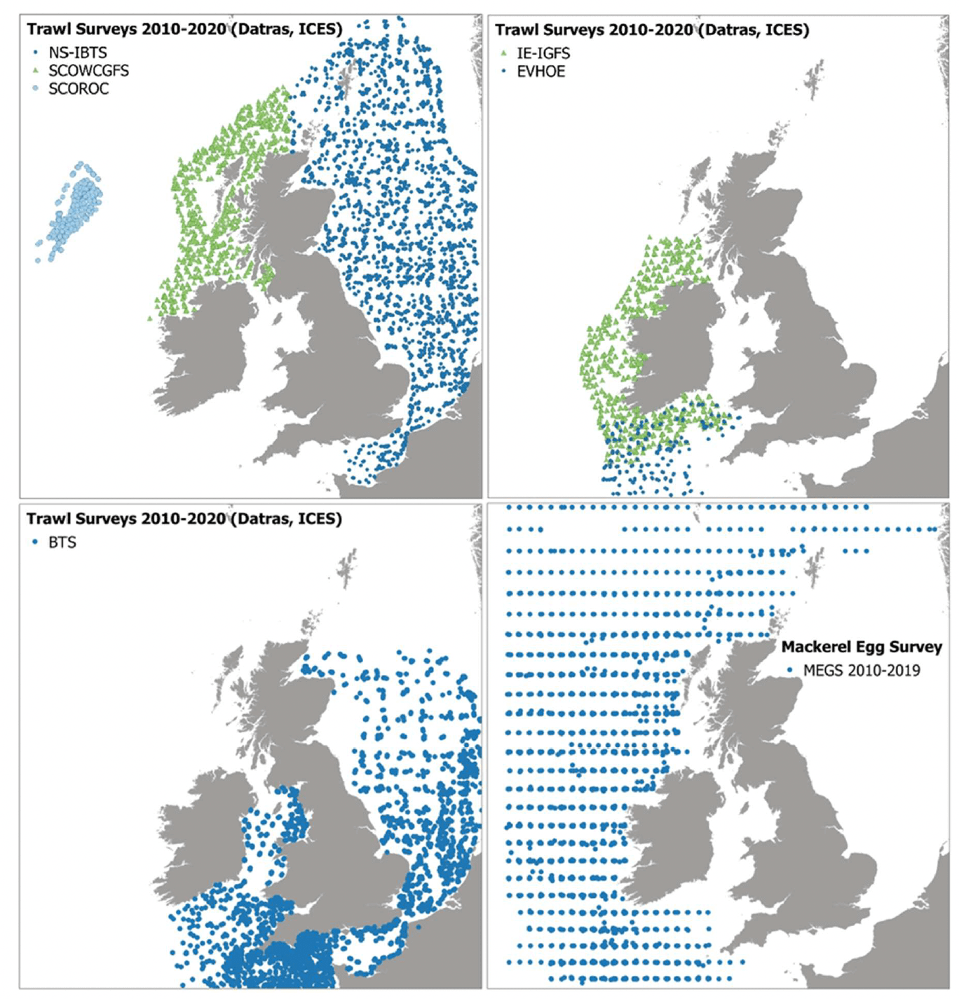
Raw data (species CPUE as number per hour per length class and hauling information) were obtained from DATRAS^[5]5, the online Database of Trawl Surveys maintained by the International Council for the Exploration of the Seas (ICES). The selected surveys for the period 2010 - 2020 included the International Bottom Trawl Surveys (IBTS) and Beam Trawl Surveys (BTS) undertaken by different countries under ICES coordination. IBTS included the North Sea International Bottom Survey (NS-IBTS), Scottish West Coast Groundfish Survey (SCOWCGFS), Scottish Rockall Survey (SCOROC), Irish Ground Fish Survey (IE-IGFS), and Evaluation Halieutique Ouest Europeen (EVHOE). IBTS data were considered more suitable to model demersal and pelagic species (with variable confidence), while BTS data were used to model flatfish.

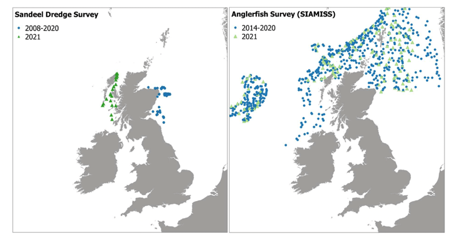
Even though the lesser sandeel, Ammodytes marinus was caught in IBTS and BTS, these survey methods are not considered to provide reliable estimates of sandeel abundance (Ellis et al. 2012, Wright et al. 2019). Therefore, alternative survey data were explored. Data on haul locations and CPUE (catch per hour, and also per age class) were obtained for the annual dredge survey undertaken by Marine Scotland Science in December at sandeel fishing grounds off the Firth of Forth and Turbot Bank (in Sandeel Area 4, east coast of Scotland, where the largest of the sandeel stocks in Scottish waters is and there is an active fishery for it). The dataset also contained data from surveys on the west coast of Scotland in 2021 that were used for map validation (see section 2.4.1). Data in this dataset are reported for generic "sandeel", without distinction by species. However, most of the catches consist of the lesser sandeel Ammodytes marinus (ICES 2010), this species being the most abundant species of sandeel found in Scottish waters, and therefore the data and resultant outputs were considered as representative of this species.

Data on haul characteristics and anglerfish (Lophius piscatorius) CPUE by length class were obtained from Marine Scotland Science for the Scottish-Irish anglerfish and megrim industry-science survey (SIAMISS) undertaken to monitor the Northern shelf anglerfish stock in subareas 4 and 6, and division 3.a (North Sea, Rockall and West of Scotland, Skagerrak and Kattegat). Data from this survey were prioritised for the modelling of anglerfish, as SIAMISS survey is considered more effective than other IBTS surveys (e.g. NS-IBTS) at catching anglerfish of the size considered in this study (Danby et al. 2021).

Data on haul characteristics and egg CPUE were obtained for mackerel, Scomber scombrus from the ICES Eggs and Larvae database^[6] for the Mackerel and Horse Mackerel Egg Survey (MEGS) in the Northeast Atlantic. The spatial and temporal distribution of sampling in this survey programme is designed to ensure an adequate coverage of the species spawning areas, with sampling effort being targeted at producing estimates of stage 1 (early development stage) egg production.

A summary of the data availability and methods for the above-mentioned surveys is given in Table 2, with the survey locations mapped in Figure 4 and Figure 5. Further details (metadata to MEDIN standard) of the selected datasets for the project are given as attached Excel worksheets including metadata for both collated raw survey datasets (worksheet 'EFH- SG2022_Raw survey datasets_Metadata_MEDIN format') and processed data for input into EFH modelling ('EFH-SG2022_Processed survey data for modelling_Metadata_MEDIN format').

Table 2. Fish surveys used to collate data for the EFH modelling.

Survey	Year (1)	Quarter	Gear (2)	Country	Reference
International Bottom Trawl Survey (IBTS):	as detailed below:	GOV	GOV		ICES 2017, 2020
NS-IBTS	1965-2021	Q1, Q3		Various (3)
SCOWCGFS	2011-2021	Q1, Q4		Scotland
SCOROC	2011-2021	Q3		Scotland
IE-IGFS	2003-2021	Q4		Ireland
EVHOE	1997-2021	Q4		France
Beam Trawl Survey (BTS)	1985-2021	Q1, Q3	BT (4/7/8m)	Various (3)	ICES 2019a
Sandeel dredge survey	2008-2021	Q4 (Dec, +Nov in 2020)	Modified scallop dredge	Scotland	ICES 2010
Northern Shelf Anglerfish Survey (SIAMISS)	2013-2021	Q2, Q4	Bottom trawl	Scotland	Fernandes et al. 2007, ICES 2018
Mackerel Egg survey (MEGS)	2010, 2013- 2019, 2021	All quarters	Bongo or 'Gulf type high-speed' samplers (national variants (4))	Various (4)	ICES 2019b

Table footnotes: ⁽¹⁾ Data within the decade 2010 - 2020 were selected for the analysis in this study. ⁽²⁾ GOV, Grande Ouverture Verticale bottom trawl; BT, Beam trawl (4m BT used by England and Belgium, 7m BT by Germany and 8m BT by the Netherlands). ⁽³⁾ NS-IBTS: Denmark, Germany, France, England, Scotland, Netherlands, Norway, Sweden; BTS: Belgium, Germany, England, Netherlands. ⁽⁴⁾ Bongo used by Faroes and Iceland; Gulf VII by Faroes, Iceland, Scotland, Ireland, Netherlands, Norway; Nacktai (modified Gulf VII) by Germany.

Form the collated surveys, data were selected for inclusion in the models if they were within the 2010 - 2020 period at the desired geographical location (Longitude <5 deg. E and Latitude ≥49 deg. N).

Data for life stages relevant to the modelling of individual species and their EFH were identified based on the criteria summarised in Table 3. The relevant seasonality for the occurrence of the different life stages and the cut-off size (body length) for juveniles were identified based on size-frequency analysis of the survey data and validated through the literature review (see Annex 1). Juveniles were preferably identified as 0-group individuals (i.e. individuals in their first year of life), where possible. However, in some instances, 1-group individuals (i.e. individuals in their second year of life) were included with the choice of the cut-off size in order to increase the dataset size and allow modelling. Despite this, data available were insufficient for some species which could not be modelled (Table 3).

For gadoids in the IBTS surveys, Spawning Maturity Age-Length Keys (SMALK) were available^[7] and were used to discriminate catches of spawning adults ('running' adults in Table 3). The size frequency distribution of individuals by maturity stage was analysed for the different surveys. The relevant season (quarter) for which spawning catch data were analysed was selected based on the following conditions for data in SMALK: >1000 observations available, >15% of individuals being mature (in spawning, spent or resting condition) and mostly in spawning/spent condition (with the presence of individuals in spawning condition as a minimum). The relative size frequency of individuals in spawning or spent conditions (maturity stages III/63 or IV/64, respectively) as derived from SMALK data was applied to the survey dataset to distinguish catches of adults at 'running' stage based on size class.

For burrowing species such as lesser sandeel A. marinus and Nephrops, individuals of any size or life stage were considered, with the seasonality reflecting predominant emergence patterns of the species from their burrows (e.g. during winter for sandeel) and/or the period of the year when catches in the surveys were maximized.

Table 3. Criteria for the selection of data relevant to the life stage of interest from survey data.

Common name	Life stage	Season	Life stage selection criterion (1)	Data source	Modelled
Lesser sandeel	any size/stage	Q4	-	Sandeel dredge survey	Yes
Nephrops	any size/stage	Q1+Q3 +Q4	-	IBTS (NS-IBTS, SCOWCGFS, SCOROC, IE- IGFS, EVHOE)	Yes
Plaice	Juvenile, 0-group, recently metamorphosize d	Q3	Body size (length): 4 cm to 12 cm	BTS	Yes
Lemon sole	Juvenile, 0-group	Q3	Body size (length): 3 cm to 15 cm	BTS	Yes
Common sole	Juvenile, 0- and 1-groups	Q3	Body size (length): 3 cm to 25 cm	BTS	Yes
Anglerfish	Juvenile, 0- and 1-groups	Q2	Body size (length): 12 cm to 28 cm	SIAMISS	Yes
Whiting	Juvenile, 0-group	Q3+Q4	Body size (length): 12 cm to 16 cm(Q3) / 20 cm(Q4)	IBTS (NS-IBTS, SCOWCGFS, SCOROC, IE- IGFS, EVHOE)	Yes
	'Running' adult	Q1	Adults at spawning or spent stage (2)	IBTS (NS-IBTS, SCOWCGFS)	Yes
Cod	Juvenile, 0-group	Q3+Q4	Body size (length): 8 cm to 19 cm(Q3) / 25 cm(Q4)	IBTS (NS-IBTS, SCOWCGFS, SCOROC, IE- IGFS, EVHOE)	No (3)
	'Running' adult	Q1	Adults at spawning or spent stage (2)	IBTS (NS-IBTS, SCOWCGFS)	Yes
Haddock	'Running' adult	Q1		IBTS (NS-IBTS, SCOWCGFS)	Yes
Norway pout	'Running' adult	Q1		IBTS (NS-IBTS, SCOWCGFS)	Yes
Blue whiting	Juvenile, 0-group	Q3+Q4	Body size (length): 5 cm to 19 cm	IBTS (NS-IBTS, SCOWCGFS, SCOROC, IE- IGFS, EVHOE)	Yes
Hake	Juvenile, 0-group	Q3+Q4	Body size (length): 4 cm to 19 cm	IBTS (NS-IBTS, SCOWCGFS, SCOROC, IE- IGFS, EVHOE)	Yes
Saithe	Juvenile, 1-group	Q3+Q4	Body size (length): 18 cm to 33 cm	IBTS (NS-IBTS, SCOWCGFS, SCOROC, IE- IGFS, EVHOE)	No (3)
Sprat	Juvenile, 0-group	Q3+Q4	Body size (length): 2.5 cm to 9 cm(Q3) / 9.5 cm(Q4)	IBTS (NS-IBTS, SCOWCGFS, SCOROC, IE- IGFS, EVHOE)	Yes
Mackerel	Juvenile, 0-group	Q1+Q4	Body size (length): 12 cm to 22 cm(Q4) / 24 cm(Q1)	IBTS (NS-IBTS, SCOWCGFS, IE- IGFS, EVHOE)	Yes
	Eggs, early stage	Q2+Q3	Eggs at early development stage (EG1)	Mackerel Eggs survey (MEGS)	Yes
Long finned squid	Juvenile, immature/recruit s	Q3+Q4	Body size (length): 1 cm to 15 cm	IBTS (NS-IBTS, SCOWCGFS, SCOROC, IE- IGFS, EVHOE)	Yes
Common skate	Juvenile, 0- and 1-groups	Q4+Q1	Body size (length): 13 cm to 40 cm	IBTS (NS-IBTS, SCOWCGFS, IE- IGFS, EVHOE)	No (3)
Thornback ray	Juvenile, 0-group including some 1- group individuals	Q1	Body size (length): 12 cm to 25 cm	IBTS (NS-IBTS, SCOWCGFS)	No (3)
Spotted ray	Juvenile (4)	Q4+Q1	Body size (length): 8 cm to 33 cm	IBTS (NS-IBTS, SCOWCGFS, IE- IGFS, EVHOE)	No (3)
Spurdog	Juvenile, newborn	Q1	Body size (length): 12 cm to 32 cm	IBTS (NS-IBTS, SCOWCGFS)	No (3)

Table footnotes: ⁽¹⁾ For juveniles: minimum body size in the catch data and maximum (cut-off) size for juveniles based on literature review and size frequency analysis of the survey data. ⁽²⁾ Maturity stages III/63 + IV/64 as based on SMALK (Spawning Maturity Age-Length Keys) available for IBTS data. ⁽³⁾ Too few occurrences of the species life stage in the surveys (<250 hauls in total, with aggregations in <100 hauls). ⁽⁴⁾ No information on juvenile size or seasonality was available from the literature. This was derived from the size frequency analysis of the survey data based on the smaller size cohort represented in the catches for the species.

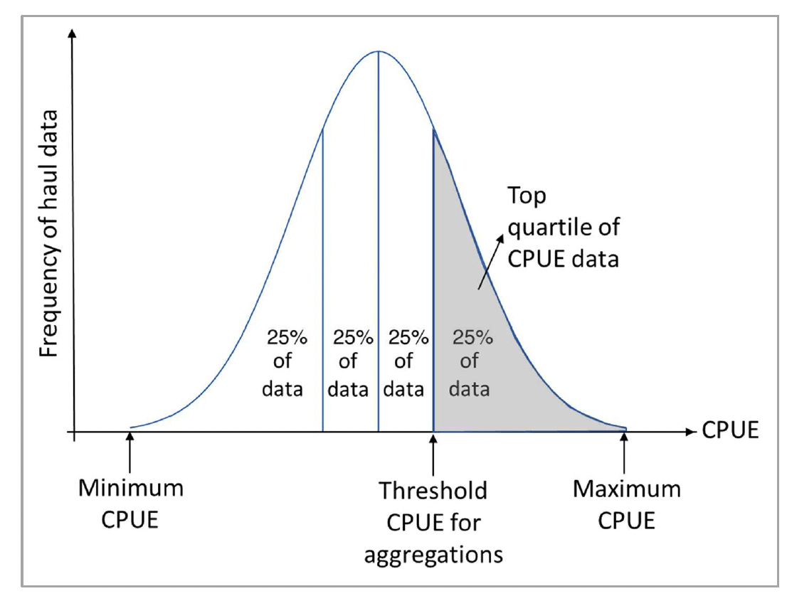
Aggregations of the species/ life stages of interest were identified based on the density (CPUE) of the catches in hauls where the species/life stage occurred, similarly to the approach used in Aires et al. (2014). A threshold value was identified as the minimum CPUE in the top quartile of the CPUE distribution of all hauls where the species/life stage was present for each survey type (Figure 6). Catches (for the selected species/life stage) with CPUE above the threshold value were identified as presence of aggregations, whereas absence of aggregations was determined where the species/life stage was present in the catch with CPUE below the threshold value. The use of presence/absence of aggregations allowed to reduce the variability in the data due to differences in sampling methodology between surveys (including gear and vessel performances) before modelling.

For most of the benthic/demersal species considered, survey types were distinguished based on the combination of Survey and Country as per Table 2 (for BTS, this also allowed to distinguish catches from different sized BT), whereas data across all years were considered given the lower interannual variability in these catches.

For pelagic species (sprat and mackerel juveniles from IBTS and mackerel eggs from MEGS), a higher interannual variability of the catch data was observed, and therefore the aggregation calculations were undertaken on a year-by-year basis for the different survey types (for MEGS data, the latter were distinguished based on gear type and country as per Table 2). In addition, the following criteria were also applied when identifying aggregations of pelagic species from IBTS: (i) a CPUE <10 individuals per haul per hour was never considered as an aggregation, even if within the top quartile; (ii) a CPUE >500 individuals per haul per hour was always considered as an aggregation, even if out of the top quartile.

2.2.2 Environmental data

As guided by the literature review and findings of previous projects (e.g. MMO 2013), a range of environmental data layers were collated to characterise the physical, chemical, and biological parameters for the UK marine environment which may be important in

determining important habitats of the target fish species at their various life stages. Datasets were chosen using criteria including geographical extent, relevance to target species (both benthic and pelagic), temporal representation, spatial resolution and confidence. Full details (metadata to MEDIN standard) of the selected data layers for the project are given in the attached Excel worksheet 'EFH-SG2022_Input+Output data layers_Metadata_MEDIN format', but are summarised in Table 4.

Environmental data layers were sourced which covered UK waters and, as far as possible the geographical extent of the fish survey data used for the project. In some cases, it was necessary to combine compatible or overlapping data products to increase geographical coverage or to include the presence of habitats which may not be specifically listed for protection (e.g. Annex 1, Habitats Directive) or as threatened or declining (e.g. OSPAR). For example, the presence of particular habitats that may influence the occurrence of a fish species in an area was measured by compiling composite datasets to represent the best geographical coverage of Sandbanks, Structured habitats (including reefs (various types), mussel/oyster beds, Sabellaria^[8], Lophelia, corals, rocky walls, coral gardens etc.) and Vegetated habitats (including kelp and seaweed, maerl beds, seagrass beds). For simplicity, specific habitats within each data layer were reduced to describe only presence or absence of the umbrella habitat type.

Data for temporally variable parameters (including temperature, salinity, net primary production and mixed layer thickness) were sourced as monthly averages to match the timing of fishing events. These data layers were available for the whole ten-year period considered in this study (2010 – 2020) with extensive UK-wide marine coverage, which allowed a matching between the environmental data and the fishing events for >98% of the data. Monthly environmental data were then processed further to represent seasonal averages appropriate for important life stages of certain species.

Fish survey location data were reduced to single points using the haul centre location, or either shoot location or haul location where both coordinates were not available. In most cases, environmental data were extracted directly for each survey point location for the model calibration. However, as the hauls in the survey datasets integrated over a trawling distance of up to 5 km, for some environmental parameters which had potential to give variable and potentially misleading values over a 5 km distance, either an average value or a predominant feature category within a 5 km buffer of the haul central point was extracted (Table 4).

Table 4. Environmental variables used in the models and their source data layer, with indication of their calculation for model calibration (based on survey data points) and prediction (based on grid, see section 2.2.4).

	Environmental Variable (Variable name and unit)	Source Layer	Model
			calibration (survey locations)	prediction (5 x 5 km grid)
Geo-morphology	Distance from coast (high water level) (Dist, m)	EMODnet	at survey point	at grid cell centre
	Depth (Depth, m)	EMODnet Bathymetry 2020	at survey point	mean within grid cell
	Slope (Slope, degrees)	(Derived from bathymetry data)	mean slope across 5 km buffer containing survey point	mean slope within grid cell
Habitat	Substratum type (Substr, see Table 5 for classes)	EMODnet Seabed Habitats 2019	predominant class within 5 km of survey point	predominant class within grid cell
	Presence of Sandbank Habitat (SandbH01, class 0/1)	Combination of: OSPAR 2020, EMODnet Seabed Habitats 2019, GEMS 2019	presence within 5 km of survey point	presence within grid cell
	Presence of Structured Habitats (StructH01, class 0/1)
	Presence of Vegetated Habitats (VegH01, class 0/1)
Energy	Currents, kinetic energy at seabed (CUR, N m2/s)	EMODnet 2017	at survey point	mean within grid cell
	Waves, kinetic energy at seabed (WAV, N m2/s)	EMODnet 2019
Water quality	Sea Surface Temperature (SST, °C)	E.U. Copernicus Marine Service	at survey point and mean for relevant month and year of survey	mean within grid cell and for relevant season within 2010 - 2020 period (or for individual years, where relevant)
	Sea Bottom Temperature (SBT, °C)
	Sea Surface Salinity (SSS, PSU)
	Net Primary Production (NPPV, Carbon per unit volume of seawater, mg C m-3 day-1)
	Mixed layer thickness (MLT, m)

Table 5. Key to codes used to identify substrate classes derived from EMODnet Seabed Habitats data layer for modelling (variable "Substr"). Only substrate classes relevant to the calibration datasets are shown.

EMODnet substrate classes	Substr (codes)
Coarse substrate/sediment	Coarse
Sand	Sand
Sandy mud	sMud
Sandy mud or Muddy sand	sMud_mSand
Muddy sand	mSand
Fine mud or Sandy mud or Muddy sand	f-sMud_mSand
Fine mud	fMud
Mixed sediment	Mixed
Sediment	Sed
Rock or other hard substrata	RockHard
[Sabellaria spinulosa] reefs	ssReef
Worm reefs	wReef

2.2.3 Species Distribution Models

Decision tree models, specifically Classification trees, were calibrated to predict the presence/absence of aggregations of a species/life stage based on the associated environmental conditions. All analyses were conducted using R version 3.3.3 (R Core Team 2017) and the R-package "rpart" (Therneau et al. 2019).

Classification trees are a type of supervised learning algorithm that organises explanatory variables in a hierarchical way, based on their effect on the response variable. The resulting model is visually represented as a decision tree that starts from a "Root node" (the full population of observations), and, after a series of splits into pairs according to alternative specific environmental conditions (e.g. depth < or ≥ of a certain value), a final prediction of presence/absence ("Terminal node" or "Leaf") is given at the end of a "Branch". Following the splits along a branch allows to identify unique combinations of variables associated with the resulting leaf prediction, and to highlight and describe the major influencing variables as a series of branches.

Compared to other classification approaches, decision trees closely mirror human decision- making and have several advantages (De'ath and Fabricius 2000, Zuur et al., 2007). The hierarchical nature of the trees allows researchers to identify the relative importance of different explanatory variables, and to accommodate the non-linearity and interaction between explanatory variables and with missing values (which may often be present for environmental variables in the datasets). A major advantage of decision trees is also that they are intuitively very easy to understand, and the resulting algorithm (i.e., the combination of environmental ranges that can be used to predict the occurrence of aggregations of a certain life stage) can be easily applied to a new environmental scenario to obtain predictions. As a result, they can be more easily communicated to a non-expert audience and used even without any statistical preparation or package needed.

Separate datasets for individual species/life stage were prepared, including the presence/absence of aggregations in the survey hauls (response variable) and the associated environmental conditions (explanatory variables or predictors, as extracted from the environmental data layers for the survey haul locations, month and year). Each dataset was randomly divided into a train subset, including 80% of the data used for calibrating the model, and a test subset including the remaining data (20%) for model statistical validation (see assessment of model performance in section 2.2.5)

On model calibration, a preliminary analysis of collinearity was undertaken to exclude highly correlated environmental variables (with Variance Inflation Factor >10 and/or Pearson's correlation coefficient ≥0.8) from the analysis. All the remaining variables were included in the analysis, with sea bottom temperature (SBT) specifically used for modelling of benthic flatfish and anglerfish, demersal gadoids and squid, while sea surface temperature (SST) was used for modelling sprat and mackerel life stages. Full tree models obtained were pruned, where needed, through cross-validation and following the "one standard deviation (1-SE) rule" (Faraway 2006, Zuur et al. 2007).

For a more detailed description of the modelling protocol used to select the best performing model, please see Annex 2.

2.2.4 Mapping

In order to predict the models over the wider marine area around the UK, a 5 x 5 km vector grid of the study area was created. The spatial resolution of the grid was defined based on the minimum resolution of the fish survey data used to calibrate the models (i.e. considering the length of the haul along which the catch data were integrated). The spatial coverage of the grid included, as a minimum, the UK territorial waters (Figure 7).

Environmental values associated with the predictors identified by the models were extracted from the relevant data layers at the resolution of the selected spatial grid (Table 4; see also diagram (c) in Appendix A). For persistent environmental variables (spatially structured but with no temporal variability), the gridded values were extracted by averaging the data from the environmental layer within the grid cells (Depth, CUR, WAV), considering the predominant substrate category in the grid cell (by area covered) (Substr) or calculating the variable at the grid cell centre (Dist) or across the whole grid cell (Slope). For non- persistent environmental variables (spatially structured and with temporal variability), data layers available for the years within the 2010 - 2020 timeframe were obtained (considering the appropriate months for the seasons relevant to the modelled species/life stages) and the gridded values were extracted by averaging the data within the grid cells and across the selected season and years (SST, SBT, SSS, NPPV, MLT).

As a result, the temporal reference for the environmental scenario and the associated predictions represented in the maps corresponds to the mean seasonal conditions for the decade 2010 - 2020.

Where a mean environmental estimate was used to represent the environmental conditions within a grid cell, the associated standard deviation was also estimated for confidence assessment purposes (see Annex 3).

The environmental criteria defined by the decision tree models were applied to the gridded environmental data to obtain maps of the associated predictions. Model predictions were mapped as both probability of presence of aggregations and as predicted presence or absence class (presence is identified by the model with a probability of presence >0.5).

The model predictions were only considered valid where the environmental variables were defined (excluding areas with missing data from the environmental layers) and were within the ranges at which the species/life stage occurred in the calibration dataset. Areas that did not satisfy these criteria were masked out in the maps (shown as grey areas). It is noted that spatial coverage by the environmental data layers was often poor in areas closer to shore (especially for data layers derived from oceanographic modelling, such as SST, SBT, SSS, NPPV, MLT), hence a better assessment of these areas is provided by the habitat proxy approach, which was developed specifically for inshore areas (see section 2.3).

For some species of higher interest (e.g. lesser sandeel, Nephrops, anglerfish) additional model predictions were mapped for individual years (2010, 2015 and 2020) to assess the influence of using more accurate environmental scenarios, compared to the average scenario for the period 2010 - 2020, as a basis for the prediction mapping. Resulting maps for the 2015 scenario for these species were used as baseline for the climate sensitivity assessment exploring changes in the mapped habitats under changes in the environmental conditions consistent with climate change predictions (see section 2.5).

The spatial implementation of the models was carried out in ArcGIS v10.8.1, with Excel (Microsoft Office Professional Plus 2016) used for part of the data processing.

2.2.5 Confidence assessment

Confidence is a key element associated with models and their predictions, as it provides guidance about how much the results can be trusted. In this study the confidence associated with the predicting model as a whole (overall confidence) was estimated along with the relative confidence associated with the spatial predictions within the resulting map (spatial distribution of confidence, associated to model predictions across cells of the spatial grid).

Both overall and spatial confidence assessments were based on the results of the statistical model used to derive the spatial prediction. For the overall confidence, a metric (the F1 score; Lewis and Gale 1994) was estimated from the statistical validation of the model by applying the model to the test dataset (see section 2.2.3) and comparing the resulting predictions against the true observations in the data. The F1 score (ranging between 0 and1^[9]) measures how well the model predicts each observation into the correct class (presence or absence of aggregations), thus providing an estimate of the overall model performance. For the spatial confidence, the probability with which a class (presence or absence) is predicted in a grid cell was estimated based on the classification success as indicated for each 'leaf' of the calibrated decision tree (i.e. associated with the particular set of environmental criteria that are satisfied within the grid cell).

The above-mentioned statistical confidence was weighted by the confidence associated with the input data used to calibrate the model (to obtain overall confidence) and to obtain the mapped spatial predictions (for the spatial confidence).

For the overall confidence, this included:

• The confidence in the fish survey data used to calibrate the specific model, accounting for the ability of the survey to reliably represent the distribution of the species / life stage of interest; and
• The confidence in the environmental data used to calibrate the model, as extracted from the relevant data layers.

These two additional elements of confidence were scored according to a set of criteria reflecting sampling or mapping methodology and quality standards, timeliness and spatial coverage of the data. Where confidence maps were available for the environmental data layers, these were used to derive the scoring.

All scorings were combined into a total confidence value (standardised on a 0-1 range) associated with each model output, also taking into consideration the different weight (importance) of the different environmental variables as predictors in the individual model for the specific species/life stage.

For the spatial confidence, a similar approach was used to derive confidence rating for the individual cells of the mapped spatial grid. The statistical confidence was weighted by the confidence associated with the environmental data layers used to predict the map. In addition to spatial confidence estimates provided with the source environmental data layers, the variability of some environmental data around the mean estimate used to characterise the grid cell was also considered, along with the different importance of the variables as model predictors, as before.

The protocol for the confidence assessments is outlined in Appendix A (diagrams (c) and (d)), and further details including the scoring criteria (through expert assessment) and methods for combining all the confidence components into total confidence values for the model overall and its spatial predictions are given in Annex 3.

With particular regard to Nephrops, it is acknowledged that using the abundance of individuals occurring on the seabed (from bottom trawl catches; see section 2.2.1) to identify burrow areas (refugia) may have some limitations, due to the highly irregular patterns in burrow emergence in this species. The direct assessment of burrows occurrence (and their density) would be a more accurate indicator for the refuge habitat of the species. As this type of data (from Nephrops TV surveys) was only made available at later stage in the project, they could not be used for the model calibration for Nephrops, but they were used for validating the resulting model map (see section 2.4.1). The limitation in using Nephrops catches to indicate refugia (burrow distribution) was taken accounted for when allocating confidence to the fish survey data used in the model.

2.3 Habitat proxies

The data collated for EFH modelling (see sections 2.2.1 and 2.2.2) had poor coverage of inshore coastal areas (especially internal waters), and therefore the EFH models were limited in their ability to assess those species which may preferably use habitats in these areas as EFH. To address this gap and complement the EFH model assessment, habitat proxies were identified for species using inshore waters.

This assessment relied on the availability of sufficiently detailed information from the literature review to allow the identification of habitat types with which the species associates for specific functions (refugia, nursery, spawning). In most cases, the evidence of this association was based on the species/life stage having been found in the habitat (or associated environmental conditions), but it was rarely based on abundance (e.g. considering aggregations) or other estimates (e.g. growth and survival rates) that may contribute to define the added value of an EFH (see section 1.2). Therefore, the habitat proxies in this assessment identify more generally the functional habitat of a species (habitat B in Figure 2), but they do not necessarily correspond to EFH, although it is likely that parts of the identified habitat function as EFH for the species (habitat C as a subset of habitat B in Figure 2).The process undertaken in the habitat proxy assessment and to obtain the resulting spatial outputs is summarised as diagrams in Appendix A, with further details on the various phases of the process being provided in the sections 2.3.1 to 2.3.2 below.

2.3.1 Habitat proxy assessment

In order to ensure standardisation through the habitat proxy assessment, the EUNIS habitat classification system was used to identify habitat types. The EUNIS habitat classification is widely used, with broad scale maps being available, covering most of the UK waters, thus allowing the results of the habitat proxy assessment to be widely implemented.

Marine EUNIS habitat types defined at Level 3 and 4 were used as potential proxies, including habitat types within the EUNIS marine habitat (code A) and marine habitat complexes (code X) classes. The assessment focused on inshore waters around the UK and, therefore, EUNIS habitats classed as offshore (deeper) circalittoral habitats (usually at a depth >60 - 80 m) were excluded a priori from the assessment, along with habitat types that are characteristics of other regions (e.g. habitats exclusive to the Baltic, Mediterranean, Black Sea and Pontic regions, and ice-associated habitats). A full list of the marine EUNIS habitat types considered for the habitat proxy assessment (including habitat code and description) is given in Appendix B.

In order to undertake the assessment, a spreadsheet (species-habitat matrix) was created in Microsoft Excel (Figure 8) where EUNIS Level 3 and Level 4 habitat types were scored according to their association with a species life stage or the species as a whole, thus potentially functioning as nursery habitats (considering juveniles), spawning grounds (considering adult spawners or spawned eggs) or refugia (e.g. for sandeel). For benthic shellfish species where the different functions may be provided by the same habitat, the assessment was undertaken for the generic species' habitat. EUNIS habitat types were rows in the matrix, and the species life stage were columns (Figure 8).

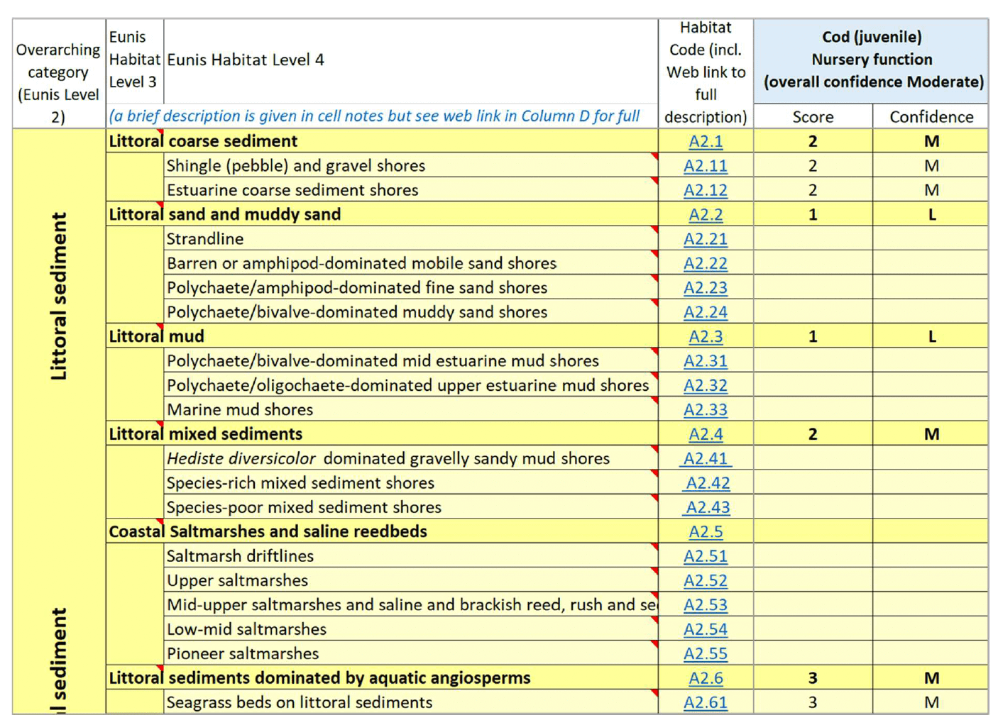
An expert assessment was applied to the information obtained from the literature review, and a score between 1 and 3 was allocated to the habitats in the matrix for each species/life stage considered. Scores were only allocated where sufficient supporting evidence of an association of that habitat with the specific life stage existed. A higher score was assigned to habitats which were identified in the literature as important/primary habitats with which the species/life stage associated (e.g. where the species/life stage was most frequently found, or with higher abundance (if this was assessed) in a study). A lower score was assigned to habitats for which there was evidence of use, but not with the same intensity (e.g. frequency or abundance) as other habitats. In a limited number of occasions, a score of 0 could be attributed to habitats for which there was definitive evidence/knowledge that they are not suitable to support a specific life stage.

A measure of confidence (Low to High) was attributed to all scores assigned to individual habitats, based on expert assessment. This reflected the frequency of evidence available across the reviewed literature which supported the assigned score for the species-habitat association (e.g. where many papers reported a strong association of a species with a habitat, a higher confidence was assigned compared to the case where only fewer papers reported a similar level of association). The ability to match environmental conditions identified in the literature as suitable for use by the species/life stage with specific habitat types (as defined at the selected EUNIS Levels 3 and 4) also contributed to the confidence assessment (e.g. a lower confidence was assigned where the habitat/environmental conditions for a species/life stage were identified in generic terms in the literature, making the correspondence with a particular EUNIS habitat type more uncertain compared to evidence on more detailed habitat/environmental preferences). An overall confidence (Low to High) was also assigned based on expert assessment, taking into consideration the amount and detail of information supporting the species assessment as a whole (across all habitats).

Scoring was prioritised at the highest habitat resolution in the matrix (EUNIS Level 4 habitats), where possible, and the score for the parent EUNIS Level 3 habitat was derived as the highest score (and associated confidence) available across the assessed EUNIS Level 4 habitats within. Where the assessment was not possible at the finer habitat resolution (e.g. insufficiently detailed information on the species-habitat association), the EUNIS Level 3 habitat was directly scored, where possible.

The scoring (and associated confidence) was initially undertaken based on expert judgement of the project team as informed by the literature review. The assessment was subsequently reviewed and validated through stakeholder consultation with fish and shellfisheries experts (see section 2.4.2 for a list of the stakeholders consulted). Stakeholders were only asked to assess the generic provision of EFH functions for a species by a habitat typology occurring in inshore areas around the entire British Isles (irrespectively of their geographic distribution).

The final species-habitat matrix resulting from this assessment was produced into an Excel tool (see attached worksheet "EFH_HabitatProxies_MATRIX)" that allows to explore the scoring and filter the matrix based on species, life stage etc.

It is of note that a study developing EFH indicators has been undertaken concurrently to this one by Natural England^[10] (Wells et al. 2022). Although the two studies have been undertaken independently, coordination in the tools used between projects was considered important for UK-wide consistency of the approach. Therefore, common structured tools for the literature review (tables) and the habitat proxy assessment (matrix based on EUNIS Level 3 and Level 4 habitats) were used. The Natural England study focused on species distributed along the freshwater-marine gradient, up to the 12 nm limit in English waters, hence had limited overlap with the species considered in this study. However, where an overlap occurred, the habitat proxy assessment undertaken for the Natural England project was also considered for the review and validation of the assessment in this study.

2.3.2 Mapping

Maps of habitat proxies for fish and shellfish species in inshore waters were produced as a spatial application of the habitat proxy assessment. The scoring system (and associated confidence) for individual species/ life stages was applied to EUNIS biotope data layers as per the assessment tool (Matrix).

EUNIS habitat datasets obtained from EMODnet were selected based on coverage of the study area and availability of habitat classification at EUNIS Level 3 and Level 4. These included broadscale data (from the EUSeaMap model) and a series of fine/medium scale layers from individual EUNIS habitat surveys. These data were processed so that habitats at the different levels of interest (i.e. Levels 3 and 4) could be layered independently. Where survey data obtained for the same area in different years were available, these were layered by EUNIS level and ordered by survey year so that the habitat classification from the most recent surveys was prioritised.

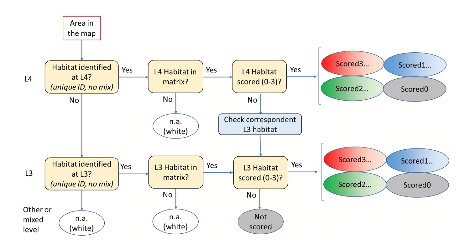
In order to fully represent the scoring (and associated confidence) from the assessment matrix, the habitat proxy maps were drawn as follows:

• Precedence was given to biotopes identified at the finer level (Level 4), which were coloured according to the combination of score and confidence received in the matrix.
• Where the Level 4 habitat was not scored in the matrix (e.g. due to lack of evidence), the score for the parent habitat at Level 3 was attributed, if assigned in the matrix.
• Any habitat in the map that was considered in the matrix, but that did not receive a score 1-3 was coloured grey in the map. This includes both habitats scored as 0 (unsuitable) or not scored (suitability unknown).
• Where the habitats in the map were identified at a coarser level than Level 3, or where habitats were classed as Level 3 or Level 4 but not assessed in the matrix (e.g. offshore (deeper) circalittoral habitats, mixed habitat classification), these were masked out in the map.

The drawing rule applied for mapping is summarised graphically in Figure 9.

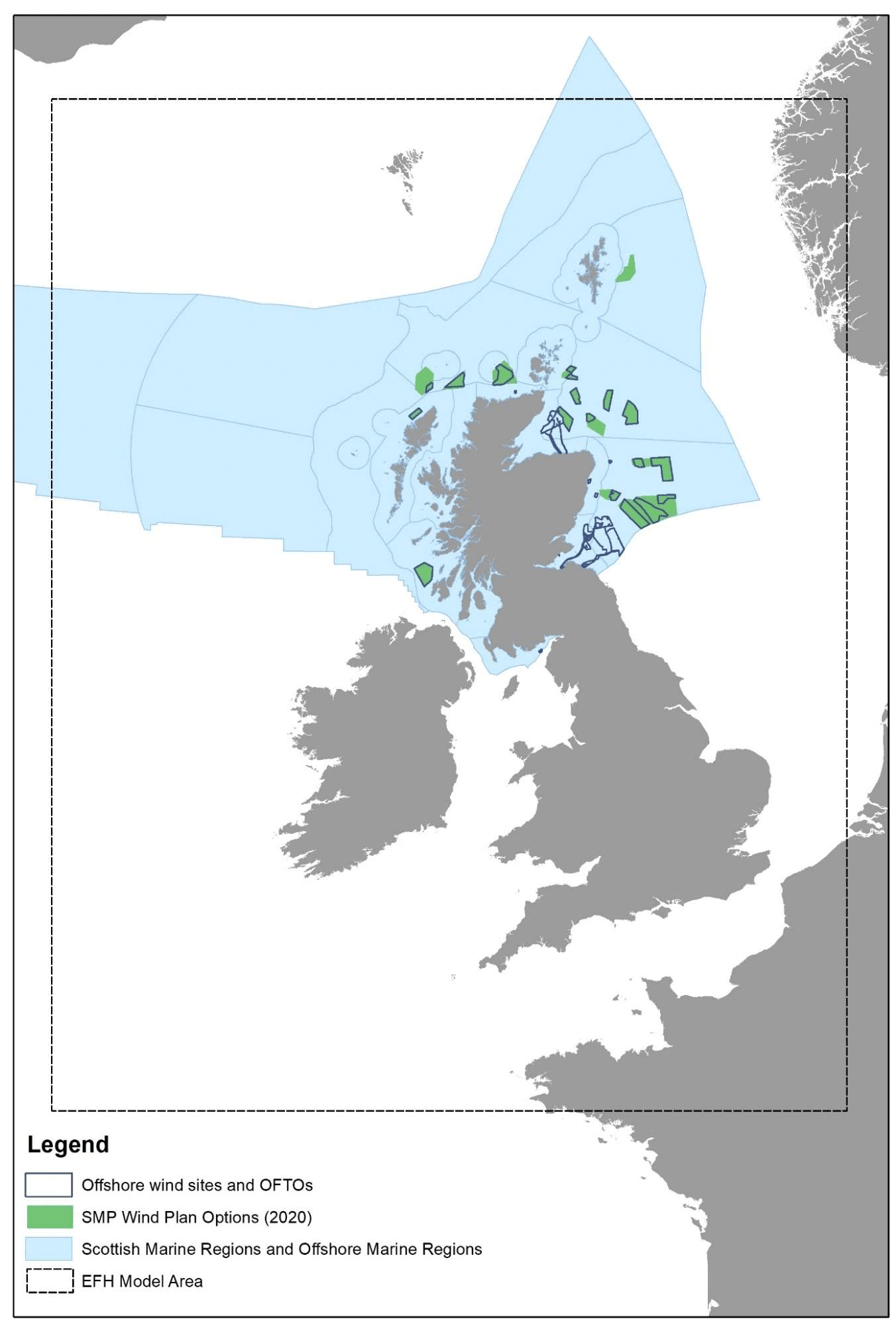
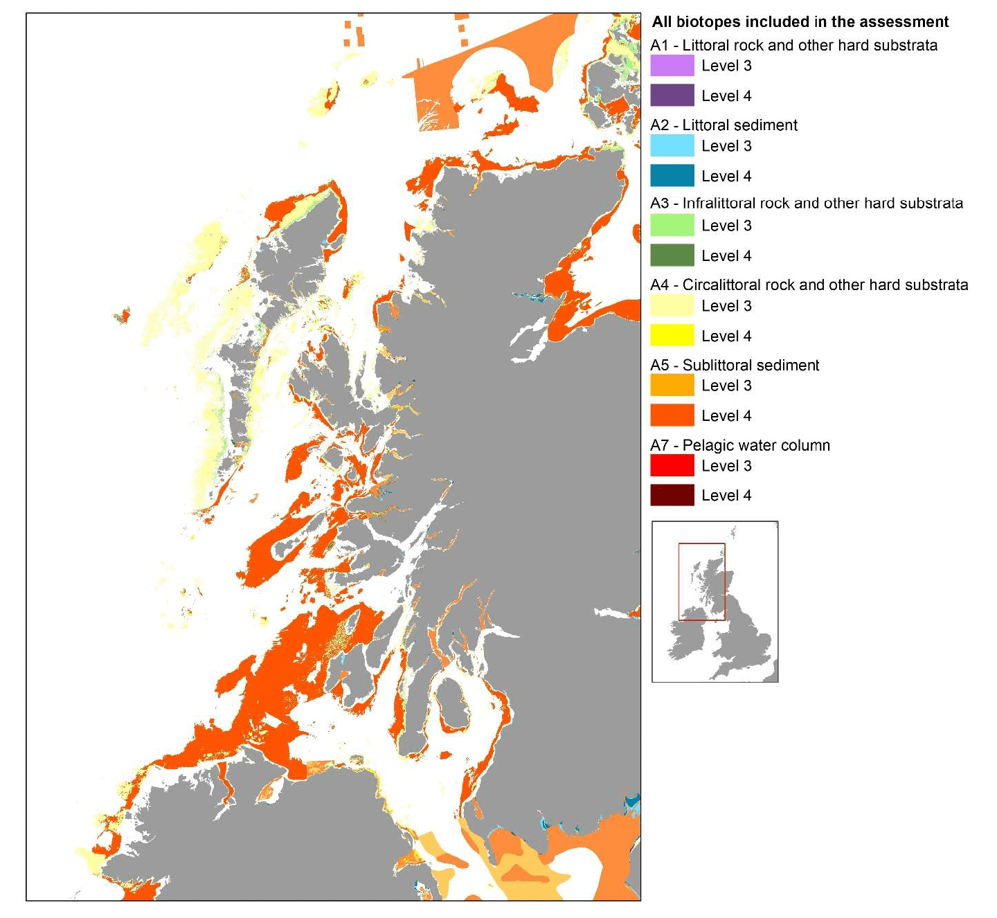
The habitat proxy assessment was applied to the EUNIS habitat data layers clipped to the wider EFH model area (Figure 7). However, due to the fine scale of the inshore habitat data, a smaller case study area was selected for mapping purposes as a demonstration of the application of the approach and to ensure the detail of biotopes at EUNIS Level 4 could be viewed. The case study covers the inshore areas on the west coast of Scotland (Figure 10). It was selected because additional data from inshore fish surveys could be obtained for this area during the project, which allowed to undertake validation of the maps thus produced (see section 2.4). Only for one species (herring spawning grounds) habitat proxy maps were produced covering all Scottish inshore waters as an example of the full extent of the results.

The integrated base layer showing the coverage and distribution of EUNIS habitats (Level 3 and Level 4, as considered in the assessment Matrix) in the case study area is shown Figure 10.

2.4 Maps validation

2.4.1 Additional survey data and evidence

Additional survey data were collated to validate the maps obtained for fish and shellfish species from both data-based models and habitat proxy approach (Table 6).

For sandeel and anglerfish, additional data were obtained from the 2021 survey undertaken within the same survey programmes that were used for the model calibration (Sandeel dredge surveys and SIAMISS, respectively). This year of data could not be included in the model calibration as some of the environmental data layers for 2021 were not available at the time of the analysis. The survey locations for these data are shown in Figure 4.

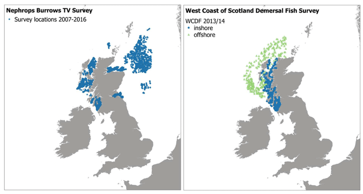
For Nephrops, additional data were obtained from the Nephrops TV surveys undertaken by Marine Scotland Science in Scottish waters (Figure 11). These video surveys are restricted to suitable Nephrops habitat (identified based on sediment characteristics or fishery VMS data), and they measure Nephrops burrow density rather than individuals, thus providing a direct assessment of the refugia resource.

Survey data from the West Coast of Scotland Demersal Fish Project (WCDF; Ramiro Sánchez et al. 2015) were also obtained for the map validation. This was a joint industry/science project (managed by Marine Scotland Science and the Scottish Fishermen's Federation Services Limited) to better understand the distribution and abundance of demersal fish on the west coast of Scotland. Offshore and inshore quarterly trawl surveys were undertaken between December 2013 and November 2014 (Figure 11). These data were used to validate both model and habitat proxy maps for different fish species (Table 6).

To ensure comparability of these additional survey data with the model prediction maps, the life stages of interest (selected by body size and season; Table 3) and their aggregations (as top quartile CPUE catches in the survey) were identified using the same method applied to the modelled data (see section 2.2.1 for details). Similarly, the top quartile of density of burrows in the Nephrops TV survey was used to identify aggregations. The distribution of aggregations identified from these additional survey data were mapped for comparison with the maps obtained from the modelling approach.

For comparison with the habitat proxy maps, the additional data from all the seasons available for the WCDF survey were considered to identify the actual occurrence of the mapped species in the case study area. The smallest cut-off body size as in Table 3 was used to identify juveniles in the WCDF survey dataset for the mapped species. The distribution of the catches from these additional survey data were mapped for comparison with the maps obtained for the west coast of Scotland from the habitat proxy approach.

Table 6. List of fish and shellfish species for which data from additional surveys were available for map validation. Seasonality and life stage for the data selection are indicated.

Common name	Life stage	Additional survey data sources
Lesser sandeel	any size/stage	Sandeel Dredge Survey 2021 (December)
Nephrops	any size/stage	Nephrops TV survey (burrows) 2007- 2016 (any season)
Plaice	Juvenile	WCDF 2013/14 (Q3 / all seasons)
Lemon sole	Juvenile, 0-group	WCDF 2013/14 (Q4)
Common sole	Juvenile, 0- and 1-groups	(1)
Anglerfish	Juvenile, 0- and 1-groups	SIAMISS 2021 (Q2) and WCDF 2013/14 (Q2)
Whiting	Juvenile, 0-group	WCDF 2013/14 (Q3+Q4/ all seasons)
	'Running' adult	(2)
Cod	Juvenile, 0-group	WCDF 2013/14 (all seasons)
	'Running' adult	(2)
Haddock	'Running' adult	(2)
Norway pout	'Running' adult	(2)
Blue whiting	Juvenile, 0-group	WCDF 2013/14 (Q3+Q4)
Hake	Juvenile, 0-group	WCDF 2013/14 (Q3+Q4)
Saithe	Juvenile, 1-group	WCDF 2013/14 (all seasons)
Sprat	Juvenile, 0-group	WCDF 2013/14 (Q3+Q4/ all seasons)
Mackerel	Juvenile, 0-group	WCDF 2013/14 (Q3+Q4)
	Eggs, early stage	WCDF 2013/14 (Q3+Q4)
Long finned squid	Juvenile, immature/recruits	WCDF 2013/14 (Q3+Q4)
Thornback ray	Juvenile, 0-group	WCDF 2013/14 (all seasons)
Spotted ray	Juvenile	WCDF 2013/14 (all seasons)
Spurdog	Juvenile, newborn	WCDF 2013/14 (all seasons)

Table footnotes: ⁽¹⁾ There were doubts on the species identification for common sole in the WCDF survey and therefore data for this species were not considered. ⁽²⁾ Data available from the WCDF survey did not allow the identification of 'running' individuals in the catches.

For herring, joint industry/science herring surveys have been undertaken in the western British Isles (ICES Divisions 6a, 7bc) since 2016 with the aim of improving the knowledge base for the herring spawning stock components in these areas and support ICES herring stock assessments (Mackinson et al. 2017, 2018, 2019, 2020, 2021). This includes acoustic surveys on known active spawning grounds, with targeted trawling to collect biological information (species confirmation, length/age, maturation state) and ground truth the acoustic data. As the information about the spawning component is given at an aggregate level by Area/Strata and cannot be disaggregated at sampling unit level, data obtained from these surveys were not directly suitable for modelling or mapping aggregations of spawning herring at the higher spatial resolution as used in the present study. Consultation with the coordinator of the surveys was undertaken instead for map validation (see section 2.4.2).

Summary information on spatial distribution of herring spawning in Scottish waters, as recently mapped by Frost and Diele (2022), combining evidence from various current and historic surveys, was also used for the map validation.

Similarly, additional evidence including, for example, known areas specifically designated or managed to protect a species (or its life stages) was obtained from the literature (also including policy documents/reports) and used to inform the map validation (Appendix C).

2.4.2 Stakeholder engagement

A component of the map validation process was based on expert knowledge through stakeholder consultation as also done (MMO 2013, 2016) or called for (Aires et al. 2014) in previous projects.

Stakeholders were selected at the beginning of the project as representatives of Government agencies involved in marine conservation and management, the fishery industry, as well as academics with experience in research on fish and shellfish habitats. Stakeholders with knowledge of the species distribution and data within Scottish waters were prioritised, but the stakeholder selection was also extended to expertise available UK- wide. The list of affiliations of the stakeholders engaged in the project is given in Table 7.

Table 7. Affiliations of the stakeholders involved in the project, with number of consultees shown.

Government agencies and their scientific advisors
Marine Scotland Directorate (Marine Scotland Science and Marine Planning and Policy divisions, incl. Marine Licensing and Operations Team (1), Fisheries Policy Team (1), MARLAB Stock Assessment and Modelling Group, Pelagic Fisheries Group), 4
NatureScot, 1 (1)
Joint Nature Conservation Committee (JNCC), 1 (1)
Marine Management Organisation (MMO), 1 (1)
Natural England (NE), 1 (1,2)
Centre for Environment, Fisheries and Aquaculture Science (Cefas; Offshore Wind Evidence and Change Programme project), 1 (1)
Industry
Scottish White Fish Producers Association (SWFPA), 1
Scottish Pelagic Fishermen's Association (SPFA; Industry Herring Survey West British Isles), 1
Scottish Fishermen's Federation (SFF), 1 (1)
National Federation of Fisherman's Organisations (NFFO), 2 (1)
Regional Inshore Fisheries Groups (RIFG), 1 (1)
Communities Inshore Fisheries Alliance (CIFA), 1 (1)
Squid Fisher (Moray Firth), 1
Academia / Consultancies
Edinburgh Napier University (WOSHH project, West of Scotland Herring Hunt), 2
University of Plymouth, 1 (2)
APEM Ltd, 1 (2)
University of Hull / International Estuarine & Coastal Specialists Ltd (IECS.ltd), 1 (2)

Table footnotes: ⁽¹⁾ Member of the Project Steering Group (PSG). ⁽²⁾ Consultees also involved as leads (Natural England and APEM Ltd) and experts (academics) in the project on EFH indicators being developed for Natural England in parallel to this project. It is of note that the Natural England project lead was also formerly Estuarine & Coastal Fish specialist on the Environment Agency's Estuarine & Coastal Monitoring & Assessment Service, hence bringing that experience to the table as well.

Stakeholders were engaged since the start of the project to also inform data sourcing (section 2.2.1). For map validation, the maps resulting from the modelling and habitat proxy approaches were shared with the stakeholders with the request for feedback on how the maps matched their expert knowledge on the species distribution (often also arising from direct experience of surveys and observations). This feedback was transferred into the final (validated) maps by highlighting the areas where discrepancies occurred. The model/habitat proxy results were examined in more detailed in those areas to identify the reason for the mismatch, where possible (e.g. whether it was due to a limitation of the modelling tool, or of its mapping using particular environmental conditions).

2.5 Implications of climate change

This section of the report explores the possible implications of climate change for the distribution of essential fish habitats (EFH) in Scottish waters. Recent literature reviews about how climate change is expected to affect the marine environment, and Scottish waters in particular, and how these affect marine species distribution informed the assessment. In addition, the EFH models developed in the project were applied to scenarios of environmental change, to better understand their sensitivity to changes in environmental conditions that are comparable with expected climate variability over the next 100 years, and therefore the implications for the spatial distribution of EFH.

Climate change has its primary cause in greenhouse gas (primarily CO2) accumulation in the atmosphere, which has been largely increased by anthropogenic inputs since the industrial era (IPCC 2014). This has caused the warming of air and water masses, with cascading effects on the ecosystem. Strong et al. (2017) summarised the effects of climate change on the marine environment, as shown in Figure 12. These include alterations of the physical, chemical, hydrological and ecological processes and properties of the marine ecosystem, and of their temporal regime (e.g. change in the frequency or clustering of rare or extreme storm events). Some of these changes affect the marine environment as a whole (e.g. temperature regime), others are more likely to affect inshore waters due to the proximity to land (e.g. river run-off inputs affecting salinity variability and contaminant and nutrient delivery to the sea), or to depth (e.g. wave action, sea level rise).

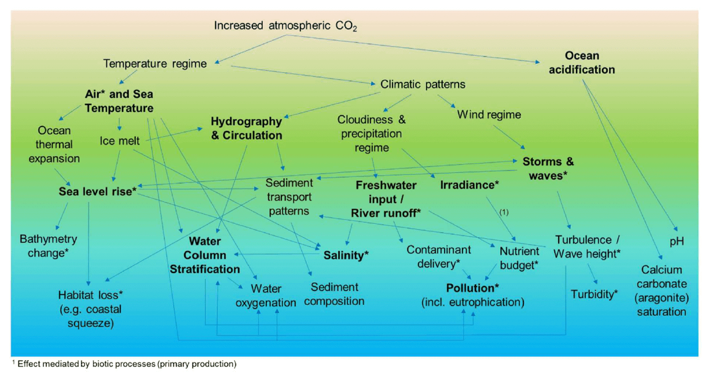
The influence of climate change on the ecology of the marine environment (also including inshore waters, such as estuaries and coastal areas) is complex and varied (Birchenough et al. 2013, Elliott et al. 2015). Fish (and shellfish) experience climate through temperature, winds, currents and precipitations, with the addition, in inshore areas, of changes in the hydrological regime, saline variability, water quality and habitat loss (Ducrotoy et al. 2019). These abiotic changes may solicit physiological and behavioural responses in the biota, altering the performance of individuals at different life stages or from different populations, influencing dispersal and recruitment and affecting species interactions within communities (see review by Ducrotoy et al. 2019 for details). Ecological effects may occur at individual, population and community levels, possibly affecting the productivity and functioning of aquatic ecosystems.

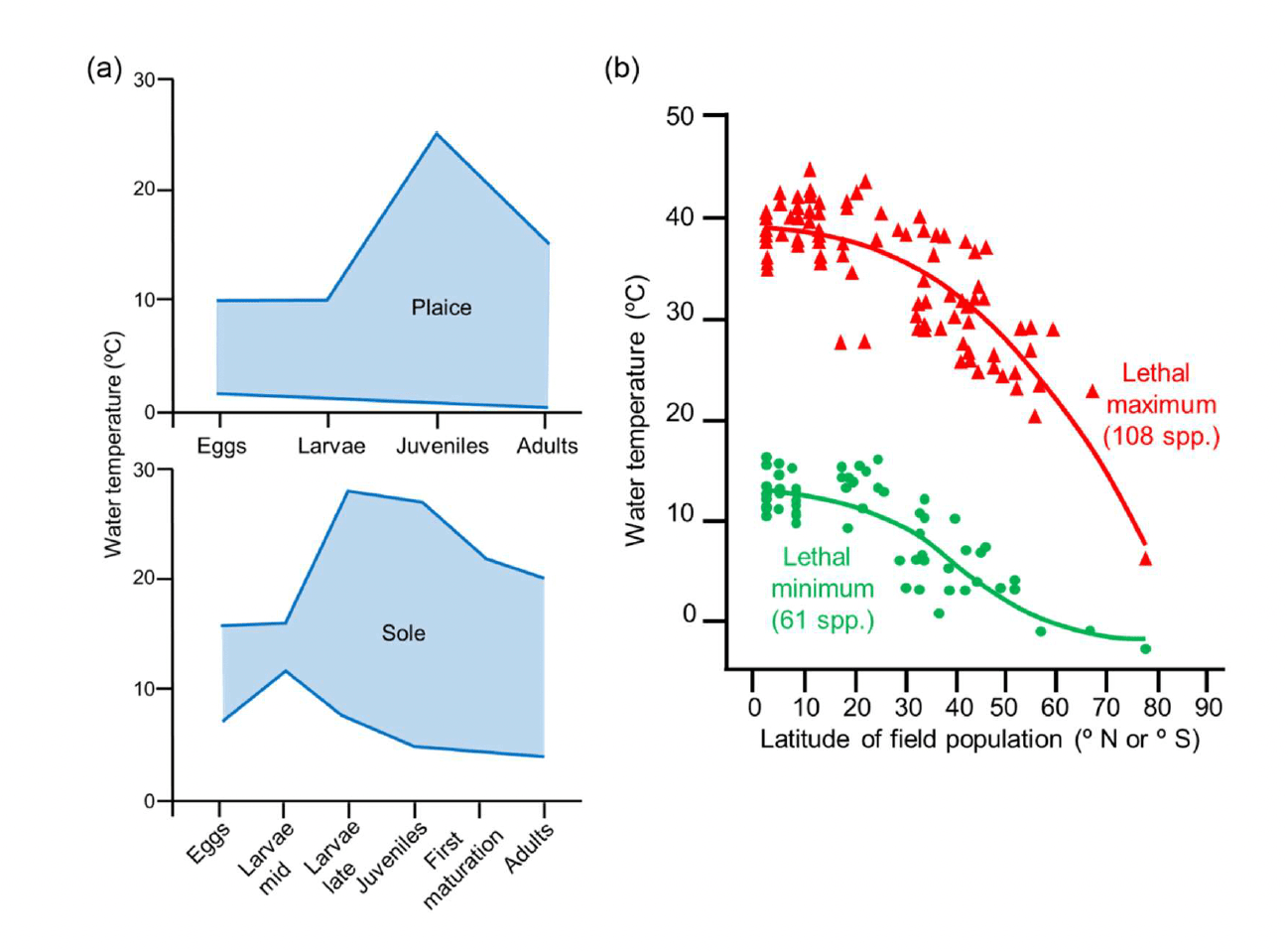
Changes in the marine environmental characteristics (e.g. water temperature, salinity, depth due to sea level rise) may alter the suitability of the habitat available to fish and shellfish in an area. The effects can vary between species or even between different life stages or populations of an individual species, for example due to the variability in their thermal tolerance range (Figure 13; Rijnsdorp et al. 2009, Freitas et al. 2010, Pörtner and Peck 2010). This may result in shifts in the geographical distribution of these species and their preferred habitats. It has been assumed that global warming, combined with local-scale processes, have led to the northward migration of marine fish along the northeast Atlantic seaboard over the last 30 years, hence affecting the distribution of their estuarine nursery grounds in this region (Nicolas et al. 2011). In the North Atlantic, the increased rate of immigration of southern species of marine fish has also been related to the warming of the water over the last 40 years (Stebbing et al. 2002). However, the effect recorded in an area may vary depending on the species, and their interaction with the local environment and physiography, and may results in variable shifts in the distribution range of different marine species in the same area (e.g. northwards or southwards, but also longitudinally or into deeper water; Perry et al. 2005, Rijnsdorp et al. 2009, Damalas et al. 2018).

2.5.1 Climate change in UK and Scottish waters

The effects of climate change on the marine environment are not geographically homogeneous, and therefore they may differently affect the distribution its biota and habitats in different areas.

Strong et al. (2017) reviewed the observed trends and future projection of climate change variables in the UK marine environment, and highlighted their spatial variability due to the local variability of physiographic and hydrographic conditions, and water masses characteristics. The variability in climate projections has also been highlighted within Scottish waters (Marine Scotland 2017a, b).

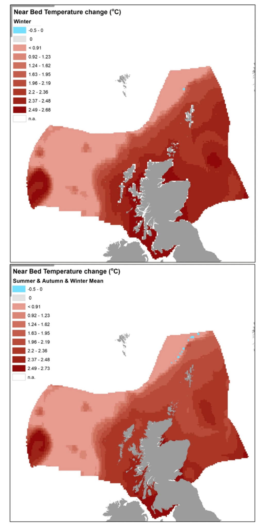
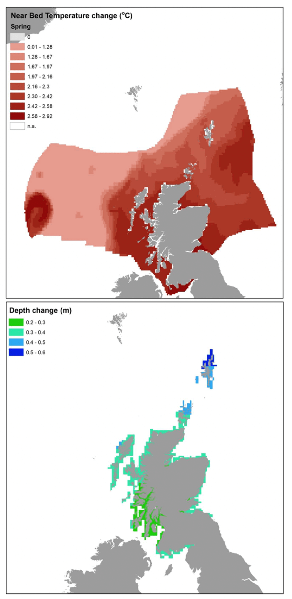
UK Climate Projections 2009 (UKCP09, for the period between 1970-80s and 2080s-90s, based on medium emissions scenario IPCC SRES A1B^[11]) indicated a higher temperature increase (by 2.5°C to 4°C at both the sea surface and sea bottom) in the southern North Sea and coastal margins of Celtic and Irish Sea, compared to the increase in the northern North Sea (by 1.5-2.5°C at the sea surface and by 0- 1.5°C at the sea bottom). According to these projections, there is marked variation both at the regional and seasonal scale within Scottish waters, for example with sea surface temperature expected to be 1°C warmer in summer north and west of Scotland compared to 2-2.5°C warmer in the remaining seasons (particularly autumn) and areas. In the deep waters surrounding Scotland, off the shelf, temperatures are projected to change very little (Marine Scotland 2017a).

While UK Climate Projections 2009 (UKCP09) indicated +12 to +76 cm absolute sea level rise (SLR) between 1990-2095 around the UK (depending on emission scenario and including land ice melt), a lower magnitude of predicted sea level rise relative to the land level was predicted in parts of Scotland compared to southern UK due to differences in isostatic adjustment (i.e. vertical land movement). Differences could be also observed within Scottish waters (Marine Scotland 2017b), the smallest sea level rise (about 30 cm by 2095, based on central estimate UKCP09 projections for 2080-90 using the medium emission scenario) was predicted in the Clyde to Skye coastal waters, as well as the inner Firth of Forth and Moray Firth, whereas increasing rise predictions over the same period were obtained for the remainder of the mainland (approximately 35 cm rise), the Hebrides and Orkney (40 cm rise), and Shetland (about 50 cm rise).

A lower incidence of thermal stratification was also predicted for waters on the continental shelf compared to the deep sea, whereas other variables showed a lower spatial variability (e.g. salinity was projected to decrease by about 0.2 salinity units across the entire northeast Atlantic and the North Sea) (Marine Scotland 2017a, Strong et al. 2017).

2.5.2 Model predictions under environmental change

To better understand how spatial predictions of potential EFH developed in the study may respond to environmental variability, decision tree models were applied to scenarios of environmental change. This exercise was undertaken for selected species of interest, including lesser sandeel Ammodytes marinus, Norway lobster Nephrops norvegicus, anglerfish Lophius piscatorius (model for 0- and 1-group juveniles) and plaice Pleuronectes platessa (model for 0-group juveniles). The models predicted aggregations of these species (at a specific stage of their life cycle in some cases) as indicators of the potential distribution

Environmental conditions in the year 2015 were used to characterise the baseline scenario for the model application, in order to obtain more accurate predictions compared to environmental conditions averaged across multiple years. The temporal reference (seasonality) to characterise the baseline environmental scenario was selected as appropriate for each specific model (Table 8).

Table 8. Environmental scenarios used to predict potential distribution of essential fish habitat for selected models (n.a., environmental change not applied as the variable was not a predictor in the specific model).

Model	Baseline scenario	Environmental change scenario
		Near Bottom Temperature (NBT) (1)	Sea Level Rise (SLR) (2)
Lesser sandeel	Dec-15	UKCP09 (winter)	n.a.
Nephrops	Q3+Q4+Q1 2015	UKCP09 (mean of summer, autumn and winter)	UKCP09
Anglerfish (juvenile)	Apr-15	UKCP09 (spring)	n.a.
Plaice (juvenile)	Q3 2015	n.a.	UKCP09

Table footnotes: Source of the mapped UKCP09 projections for Scottish waters: ⁽¹⁾ Marine Scotland 2017a; ⁽²⁾ Marine Scotland 2017b.

The scenarios of environmental change were obtained from a subset of the UKCP09 marine and coastal projections over a 100 years span, based on a medium emission scenario and, where appropriate, medium probability, as available for Scottish waters from spatial layers in Marine Scotland Maps NMPi (National Marine Plan Interactive^[12]). Specifically, the data layers for the following projections were sourced from NMPi:

• UKCP09 Projections - Change in near bed temperature (°C) by 2085, compared to 1975, medium emissions scenario for 1) winter; 2) spring; 3) summer; and 4) autumn.
• UKCP09 Projections - Rise in Relative Sea Level (cm), 2095 compared to 1985, medium emissions scenario and with medium probability.

Data were extracted for these maps into the model grid and the change (Figure 14) applied to relevant environmental variable (sea bottom temperature (SBT) or Depth) under the baseline scenario (year 2015), considering the relevant seasonality for the species considered (Table 8). As the relative sea level rise (SLR) predictions were only given for the Scottish coastal waters, the depth change was only applied to coastal grid cells where this was assessed, whares water depth was left unchanged (from baseline conditions) in the other grid cells.

The models for the selected species were applied to both the baseline scenario and the one accounting for environmental change, in relation to the change relevant to the specific model predictors (Table 8).