The Scottish Shelf Model. Part 2: Pentland Firth and Orkney Waters Sub-Domain

3 Hydrodynamic Model Development

3.1 Introduction

This section of the report describes the setting up of the PFOW model mesh, bathymetry and the calibration of the flow model. The version of FVCOM used was 3.6.1, with the code being compiled using the Intel Fortran and C compiler for LINUX.

3.2 PFOW flow model setup

3.2.1 Model mesh

The model mesh developed for the PFOW model has been created using the DHI MIKE 21 mesh generator. The horizontal coordinate system used has been latitude and longitude with a vertical datum of mean sea level.

A number of tools exist for generation of the mesh, including SMS and BlueKenue, however our preferred choice was the MIKE 21 Mesh generator because of its ease of use and flexibility. However later on in the study, the FVCOM grid was converted into an SMS format so that the quality checking built into the SMS mesh generator could be used. This enabled a final smoothing/editing of the mesh to be done so that it met all of the FVCOM mesh criteria.

The MIKE 21 Mesh generator requires coastline and boundary data to define the extent of the active and inactive mesh. Additional information is provided regarding the resolution required in user-specified domains. The resolution is based upon modelling experience, bathymetry gradient/resolution, geographical features and requirements for the study. Although the mesh generator is able to create meshes with triangular or quadrilateral elements, FVCOM requires only triangular elements. Mesh generation is an iterative process in order to derive a mesh that varies smoothly, with triangles that do not have angles that are too acute (less than 30 ^o), and resolution that does not require an overly small model timestep. The mesh file produced in the MIKE 21 mesh generator is in ASCII format that is easily converted into a format that can be used by FVCOM. This has been done using a FORTRAN code to read and write the data into the necessary format.

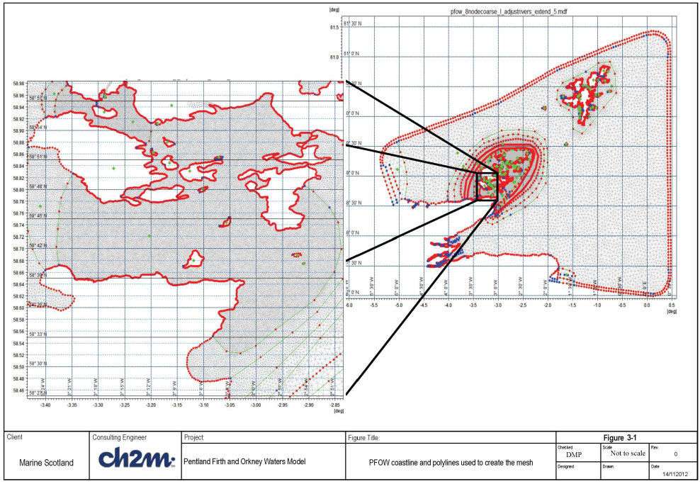
The whole PFOW model mesh is shown on the right hand side of Figure 3-1. This shows the variable resolution employed in the mesh. The resolution is much higher within the Pentland Firth and the waters in and around the Orkney Isles than further afield away from these areas of interest. The left hand image in Figure 3-1 shows a closer view of the model mesh within the Pentland Firth and Scapa Flow. Resolution in the coarser parts of the model domain away from the area of interest is approximately 2.5 to 3km, whereas within the Pentland Firth and Orkney waters the resolution is in the order of 250m, reducing to 150m in places.

Two coastline data sets have been obtained for use in this study, the Global Self-consistent, Hierarchical, High-resolution Shoreline ( GSHHS) distributed by National Geophysical Data Centre ( NGDC) in the US, and Ordnance Survey Mapping. These are discussed and attributed in Section 2.2. The coastline was resolved to between 120m-200m around the Orkney Isles and Pentland Firth (depending upon orientation with latitude/longitude. The coastline and the polylines used to define areas with different resolutions can be seen in Figure 3-1. The offshore boundaries of the model can also be seen in this Figure, it was defined to be along the continental shelf edge in the northwest and generally perpendicular to the tidal flow to the east and south. It can be seen that there is a polyline inside the outer boundary. The nodes along this line were defined so that one edge of each open boundary elements is normal to the open boundary. Although FVCOM will run without this restriction, it helps to reduce numerical noise due to high frequency wave reflection from the open boundary.

3.2.2 Model bathymetry

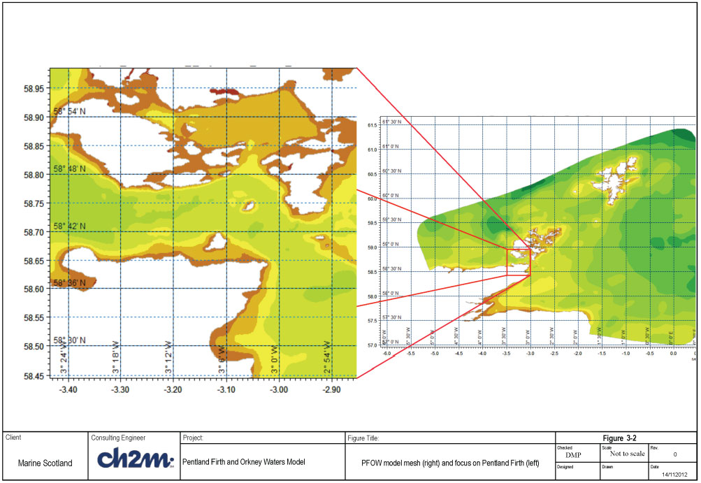
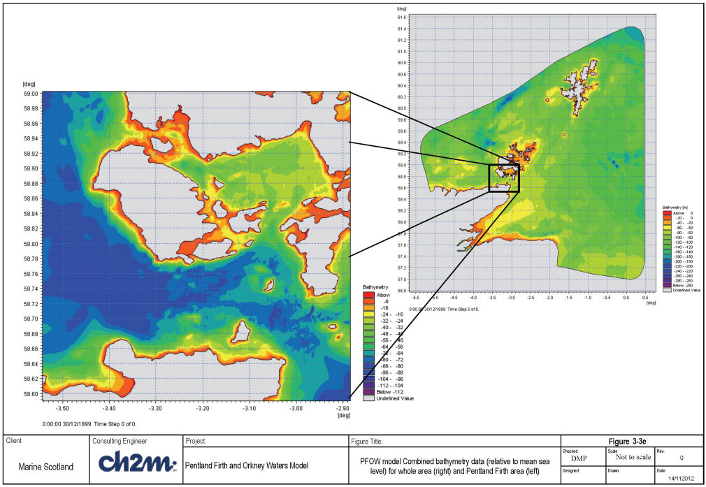
The model bathymetry was interpolated onto the model mesh presented in the preceding Section. This provides FVCOM with details about resolution and bathymetry upon which to perform its simulations. Figure 3-2 presents an overview of the bathymetry over the whole model area as well as within the Pentland Firth. This section describes the data used and the final model bathymetry taken forward for the model simulations.

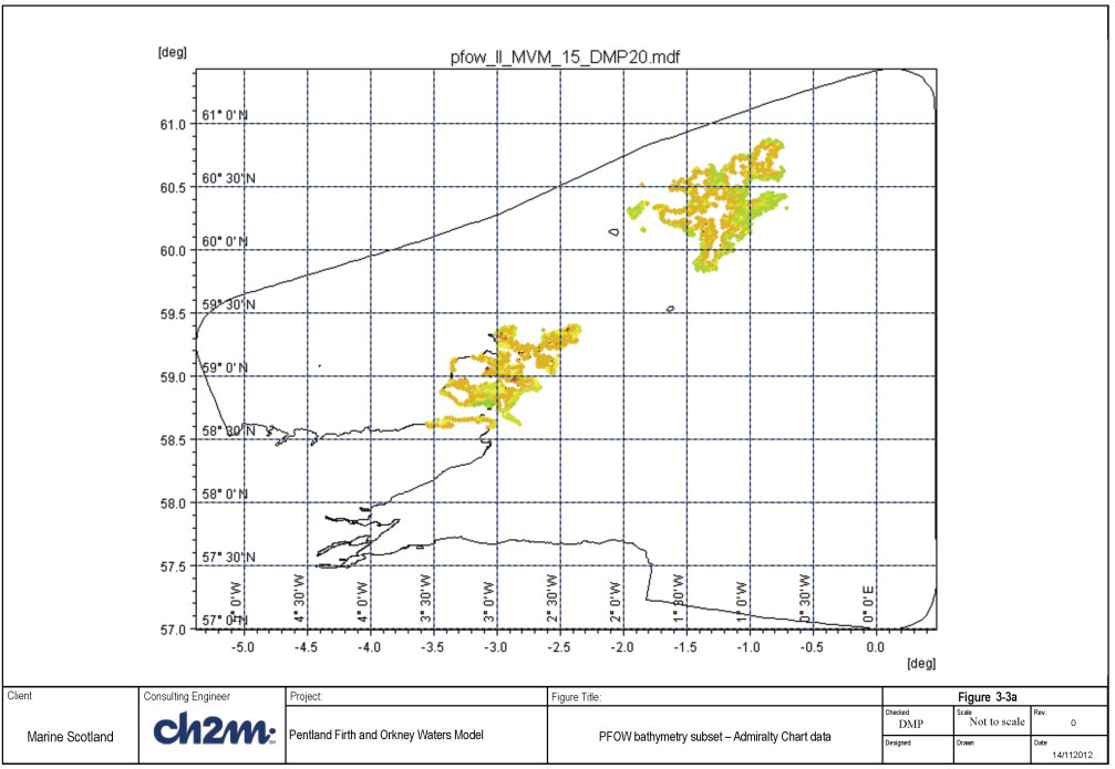
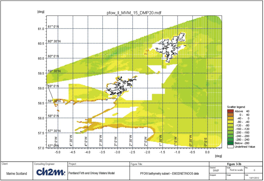
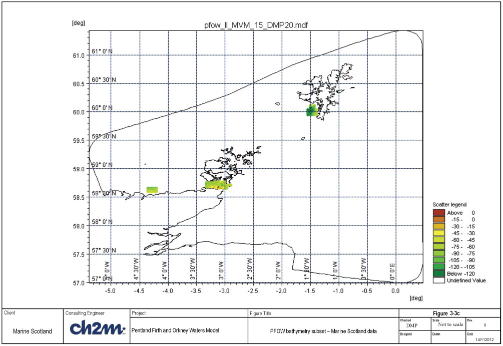
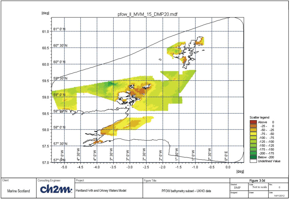
As discussed in Section 2.2, different datasets were available at different resolutions and coverage. Where possible the highest resolution data was used, this was in general from the UKHO (United Kingdom Hydrographic Office) and Marine Scotland datasets. The EMODnet/ NOOS datasets covered a wider area but had a lower resolution. There were some areas however that did not have sufficient resolution to resolve narrow waterways in sufficient detail, in these instances Admiralty Charts were digitised (under licence with the UKHO). The different datasets were converted to a common datum of Mean Sea Level ( MSL) by using conversions provided in Admiralty Tide tables that had been interpolated onto a surface. The separate datasets can be seen in Figures 3-3 a-d, and the combined dataset interpolated upon the mesh elements in Figure 3-3e.

The mesh information and the interpolated bathymetry values at the mesh nodes are saved in and an ASCII formatted Mike21.mesh file. Fortran code was written which read in this file and produced the necessary grid, depth and open boundary files required by FVCOM. When setting up the MIKE 21 mesh, it is possible to add a code to the open boundary. The FORTRAN code uses this to identify boundary nodes, which enables it to produce the open boundary files required by FVCOM.

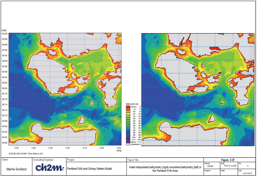
The final mesh used for the simulations presented in this report had been converted from the FVCOM grid file into an SMS format. This allowed the mesh to be adjusted to fit within the recommended FVCOM quality indices (Please see the FVCOM manual (Chen et al, 2013) for details). Additionally after carrying out some simulations it was found that the model was more stable if the bathymetry was smoothed which helped reduce steep gradients in the mesh bathymetry. The mesh bathymetry was smoothed four times using the FVCOM toolbox smoother. Figure 3-3f shows the originally interpolated bathymetry in the left frame, and the smoothed bathymetry on the right. In general all of the main features remain although some finer variations in the Pentland Firth have been smoothed out.

 

3.2.3 Boundary data

Boundary data for the model calibration and validation simulations have been derived from the NOC-L Atlantic Margin Model ( AMM). This model provides hourly water level, depth-averaged velocities, and daily temperature and salinity throughout the models vertical layers. Matlab routines were provided by NOC-L to read in the water level and temperature/salinity files. These routines were extended, so that the model boundary nodes were used to extract and interpolate the AMM model data onto the PFOW model boundaries. Water levels were produced around the PFOW model boundary at 0.25 hourly intervals from the AMM model.

In the earlier stages of the modelling, the PFOW model was run with 3 vertical layers using water levels only at the model boundaries. Although problematic initially a near 30 day simulation was achieved and the model was calibrated against data. However, with 10 vertical layers, it was not possible to get a model that would run stably (with water level boundary data only) no matter what was tried. In the end nesting boundaries were investigated in which velocities, temperature and salinity are prescribed at all the nodes associated with the elements along the open boundaries. The prescription of the velocities, rather than letting the model calculate them itself proved to be important to run the model successfully. Water levels were still prescribed as before, therefore choosing the type 2 nesting approach, rather than the type 1 where water levels are also prescribed in the nesting file. Further details on type 1 and type 2 nesting approaches can be seen in the FVCOM manual (Chen et al, 2013).

Temperature and salinity data have been extracted from the daily AMM model data and also included in the nesting file.

3.3 Flow model calibration and Validation

3.3.1 Introduction

The calibration and validation of the PFOW flow model has been undertaken in a number of stages; the first being the running of the FVCOM model (version 3.1.6) and making sure that it is stable; secondly, comparison against tides and current speeds for a period in 2001 using tidal forcing (constant temperature and salinity) and validation against currents in December 2012.

The PFOW model was originally run on a 64-core computer running Windows Server 2012 operating system. FVCOM was installed using CYGWIN, a linux emulator that runs under Windows. However there were many problems with using this approach along with using the GNU Fortran and C compilers. Therefore a virtual LINUX machine was created on the computer with 60 available cores. This was used for many of the early simulations, however we have since used a larger cluster (called EnCORE, www.stfc.ac.uk/hartree/) which has allowed us to run simulations with up to 500 cores.

The next sections describe what was required to get the model running stably, and the sensitivity tests and calibration against observed data.

3.3.2 Initial model runs

Initial runs of the PFOW model were undertaken with FVCOM version 2.7, however as soon as version 3.1.6 was obtained all effort was switched to this version. Boundary conditions were obtained for a period in 2009 from the AMM model and were used to get the PFOW model running.

Initially problems were encountered with the model crashing; these issues were tracked down to problems at the model boundary as well as internally with small elements. The model at this stage was run using 3 vertical layers. The following adjustments to the model setup were found necessary in order to obtain a stable 3-layer model.

• Some iterations were made with the model mesh to remove small elements as well as smooth bathymetry in a deep area (>200m) west of Shetland (on the offshore boundary adjacent to the continental shelf) where instabilities were observed.
• Further adjustments to the mesh bathymetry were made at the points where the open boundary met with the mainland coast. At these locations the depths were adjusted so that they did not dry out and are uniform so that any gradients did not produce instabilities.
• Bed roughness maps and horizontal mixing maps were applied to the model with increased values at the open boundary (a few elements wide) in order to damp any oscillations or instabilities. This had the desired effect without any significant impact upon the model calibration.

The vertical resolution in the model was subsequently increased to 10 vertical layers and many stability problems were encountered. As discussed in Section 3.2.3 a nesting boundary approach was adopted, making the model behave much more stably. This meant that the adjustments to the model roughness and horizontal mixing at the boundaries (using the maps) were no longer required. Likewise sponge nodes were also not required.

A period in 2009 was initially selected for the calibration period. This period was chosen as the most complete set of data for calibration and forcing the model was available (full met forcing, river flows, tides and current transects). However it soon became apparent that although there was ADCP data available in the Pentland Firth, this was only transect vessel mounted ADCP data ( VMADCP) in a small area between Stroma and the Scottish mainland on the south of the Pentland Firth. Some preliminary results were presented at a Steering Group meeting. However it became apparent that this data was not representative over the entire Pentland Firth and only provided data over a relatively short time period.

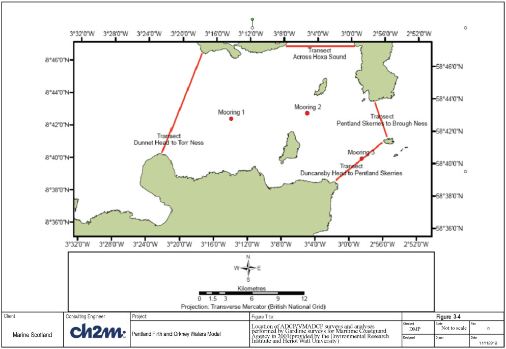
Therefore, the focus was shifted to the 2001 ADCP and VMADCP data mentioned in Section 2. This data was received from the Environmental Research Institute and Heriot Watt University, but originally collected by Gardline Surveys for the Maritime and Coastguard Agency. Figure 3-4 presents the locations of the three fixed stations and the VMADCP transects. Whereas this data provides good spatial and temporal coverage within the Pentland Firth there are some other limitations in using this data. Only wind speed and direction is available for the met forcing and there is no river flow data available from the Grid2Grid model during this period. However for the purposes of calibrating the model for tide and currents it was felt that the 2001 data was superior to the 2009 data.

Emphasis was placed upon the three fixed stations initially as these contained approximately 30 days of current measurements through the water column. These have been depth-averaged for initial calibration prior to including temperature and salinity variations at the model boundary.

Table 3-1 presents the details of the ADCP campaign, this table was taken from Table 1 in Baston and Harris (2011). It shows that the ADCP data did not provide information in the top 10m of the water column which may mean that the 'observed' depth-averaged peak speeds (calculated by depth-averaging below the 10m level in the water column) may be slightly lower than would otherwise be observed.

Table 3-1 2001 ADCP characteristics in the Pentland Firth

Location	Number of 4m bins	Deepest Bin depth(m)	Shallowest Bin depth(m)	Duration (days)	Deployment date
1	17	77	13	32.5	14/9/2001
2	17	75	11	31.25	19/9/2001
3	15	67	11	30	15/9/2001

The calibration effort at this stage has been focussed on reproducing correctly the tidal levels and flows in the model area, while keeping the temperature/salinity variation constant. Early versions of the model with 3 vertical layers were used for model calibration so as to speed up the simulations. However the final results presented in this report are for the 10 layer model unless otherwise stated.

3.3.3 Model calibration against 2001 data

The calibration described in this section has been performed with constant temperature and salinity boundaries, ten vertical layers and without the effect of meteorology or river inputs. Water levels were applied to the boundary nodes at 10 minute intervals whilst the depth-averaged velocity from the AMM model was prescribed using a nesting boundary file equally through the vertical layers. The main purpose of this calibration is to make sure current speeds and water levels are reasonably reproduced within the Pentland Firth model given the forcing from the AMM model. The Pentland Firth is highly energetic and tidally dominated and therefore it is felt that this is a valid approach prior to including other forcing terms which may be of secondary importance. In Stage 3 of this project, the regional shelf model (developed in Stage 1) is used to supply boundary conditions to the four individual case study areas developed in Stage 2. However, as the development of the Stage 1 and Stage 2 models is carried out in parallel, the boundary conditions used for the stage 2 models is derived from an external source; in this case the AMM model.

The level of calibration of the PFOW model has been determined by visual inspection of time-series comparison (speeds and water levels) as well as statistical analysis for a more quantitative comparison. A description of the statistical measures is presented later in this section. Additionally comparison against calibration guidance provided in Bartlett (1998) has also been made.

3.3.3.1 Sensitivity to bed roughness

Initial model runs (using the 3 layer model) undertaken for comparison against the 2001 timeseries data used the default bed roughness of 0.1m and a horizontal mixing Smagorinsky coefficient of 0.2. Current speeds from the model tended to under-predict the peak speeds on the flood tides at Moorings (locations) 1 and 2 - see Figure 3-4 for locations. Sensitivity to bed roughness was therefore undertaken with the aim to improve the comparison with the data. Each model was run for a period of 16 days, with subsequent analysis undertaken for the last 15 days. The model is driven by boundary conditions (water levels and depth-averaged currents) from the AMM model although no meteorological forcing has been included. This sensitivity analysis is presented in Appendix A.

The sensitivity tests to roughness presented in this current section are for the ten layer model but have made use of the earlier findings from the three layer model tests presented in Appendix A.

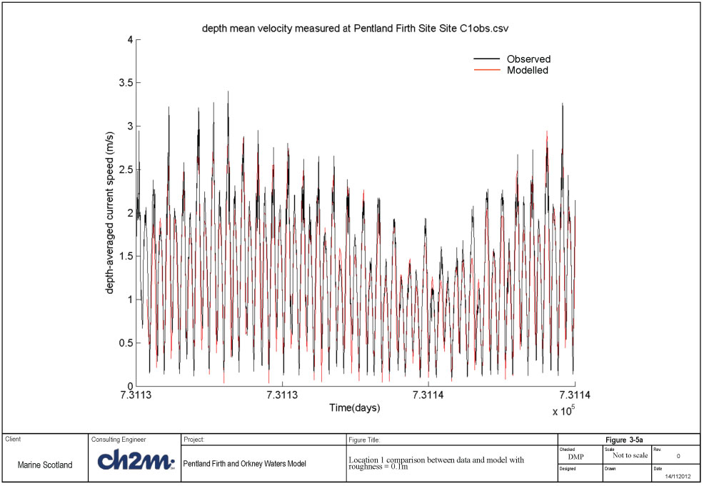
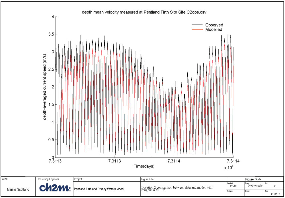
During the development of the 10 layer model it was found that using the original roughness of 0.025 produced speeds that were too high. Therefore building upon the 3 layer model results two bed roughness values were tested - a roughness length of 0.1m, and a roughness length of 0.04m. The results of the comparison of observed and modelled speeds can be seen in Figures 3-5a-c for the roughness =0.1m and Figures 3-6a-c for a roughness length of 0.04m. On each of these plots, in common with other figures in this report, the observed data is represented with a black line and the model results with a red line.

Figure 3-5a shows that at location 1 there is a significant asymmetry in the depth-averaged tidal currents (Figure 3-6d has a closer view). With a roughness length 0.1m the model tends to under predict current speeds, especially for the smaller of the two peaks in each tide. Figure 3-6a shows the same location but for a roughness of 0.04m. This shows a slight over-prediction of the highest peak currents in some instances but the lower peak is reproduced well.

Figure 3-5b shows that at location 2 there is no obvious asymmetry in the depth-averaged tidal currents. With a roughness length 0.1m the model tends to under-predict current speeds. Figure 3-6b shows the same location (Figure 3-6e has a closer view) but for a roughness of 0.04m, the match with the current speed is improved over that shown in Figure 3-5b.

Figure 3-5c shows that at location 3 there is a strong asymmetry in the depth-averaged tidal currents. With a roughness length 0.1m the model tends to under-predict current speeds for the smaller of the peaks, but over-predict the larger one on each tide. Figure 3-6c shows the same location but for a roughness of 0.04m (Figure 3-6f has a closer view), the match with the current speed is improved for the smaller of the peaks although the higher of the peaks is over predicted. It should be noted however that the ADCP data misses out the top 10m of the water column, and therefore the depth average value may in fact under-estimate the actual value.

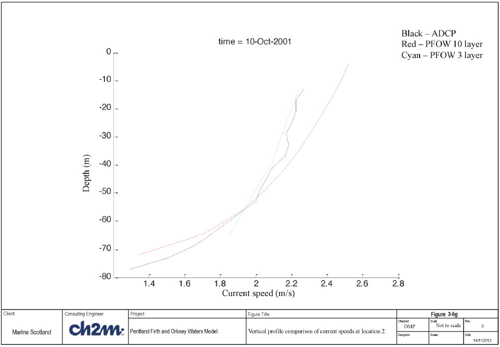
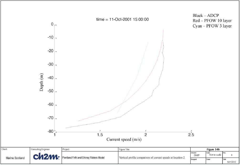
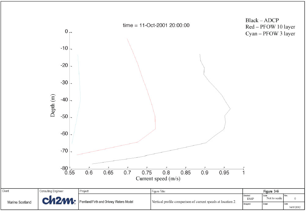
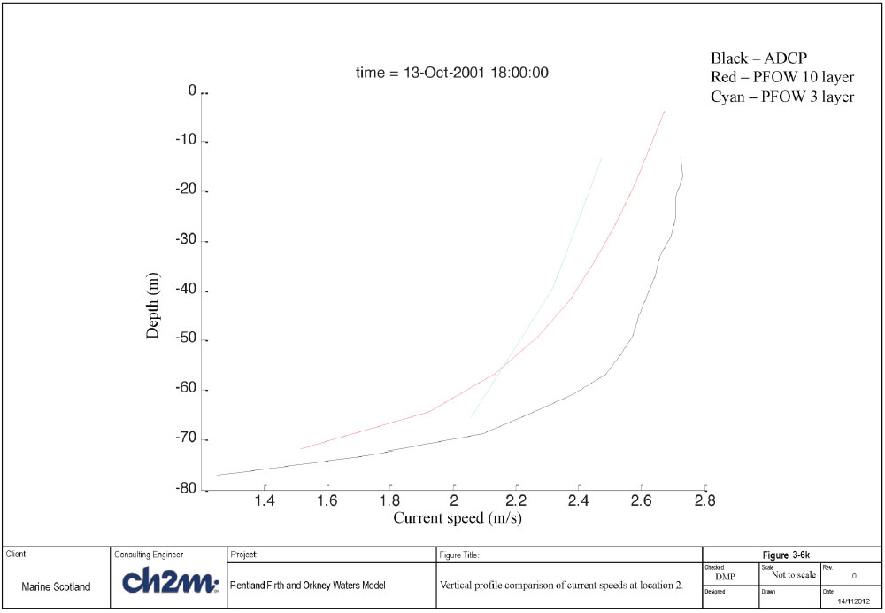
Figures 3-6g-k present comparisons of the same ADCP data at location 2 against model results but at instantaneous times through the vertical. The model results compared are for the 10 layer model and the 3 layer model. There are some differences between the model setups (10 layer model had a slightly higher roughness, and the boundary condition approach was different) and so an exact match between the two model results should not be expected. However these have been included so that the differences between the 3 and 10 layer can be seen. It should be noted that on each of these figures the axis scales differ.

What is evident from these figures is that the 10 layer model represents the lower velocities towards the bed in more detail as might be expected, and similarly for near surface speeds. The 10 layer model is able to represent the vertical variation in velocity much better than the 3 layer model. Figure 3-6i shows a time when there is a reversal in the flow, with the peak velocities in the ADCP data appearing approximately at mid depth. The 10 layer model is also able to reproduce this feature (although with lower magnitude - difficult to get phasing exactly the same) whereas the 3 layer model barely shows this feature. Although such a flow structure appears for only a short period of time during a tidal cycle, it adds confidence to the 10 layer model that it is able to reproduce this structure.

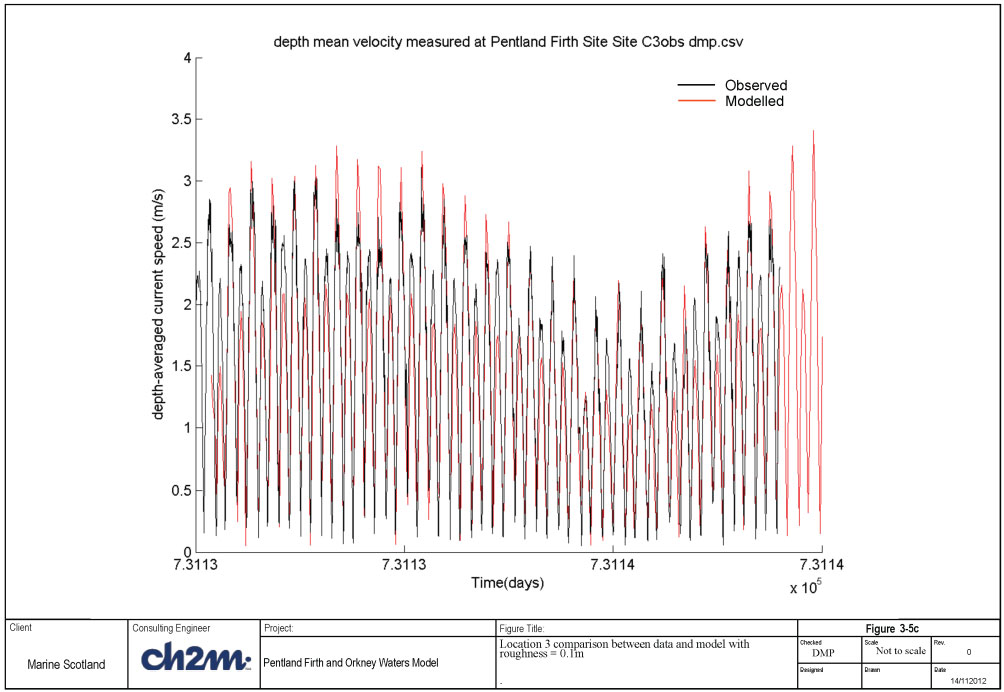
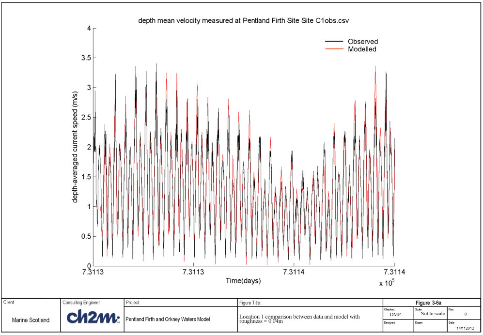
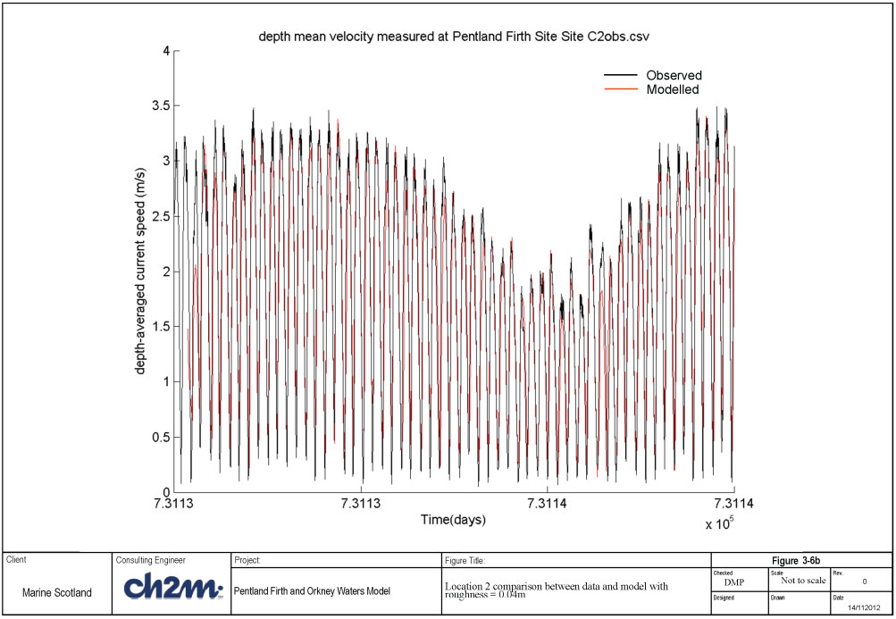
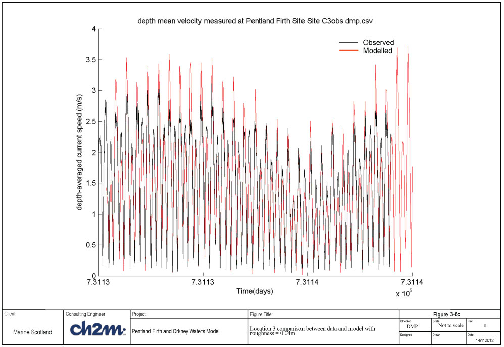
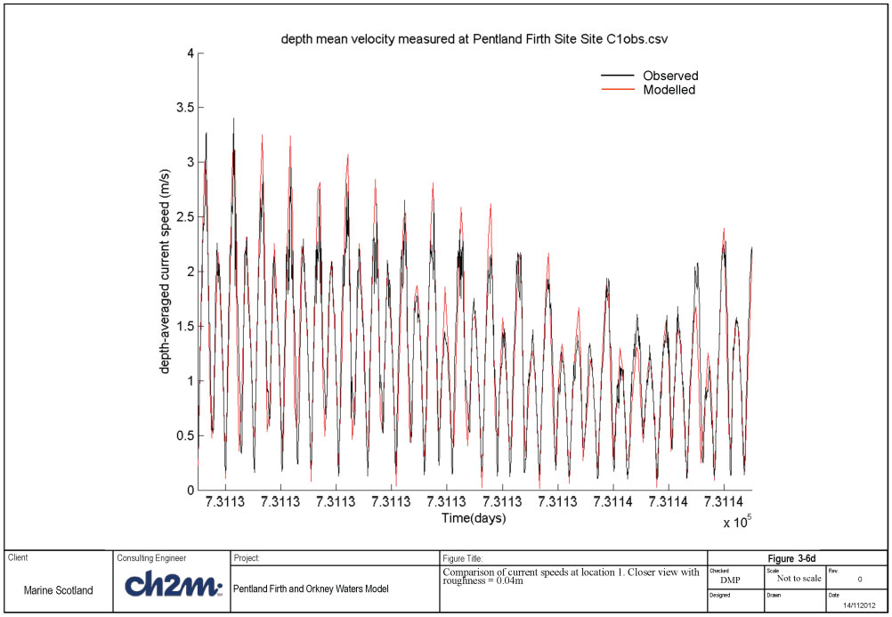
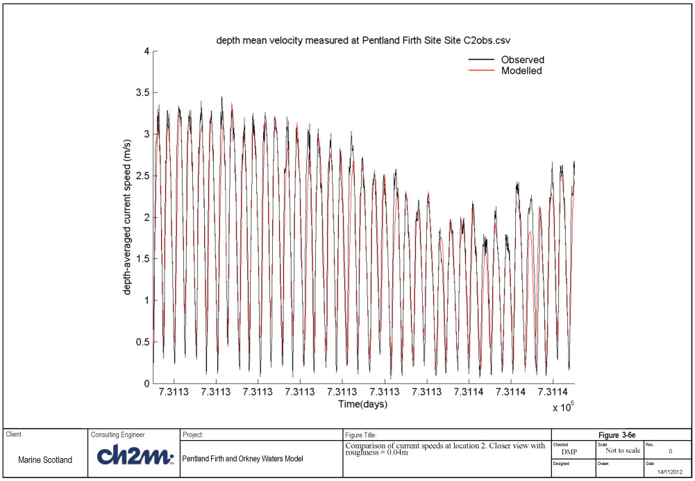
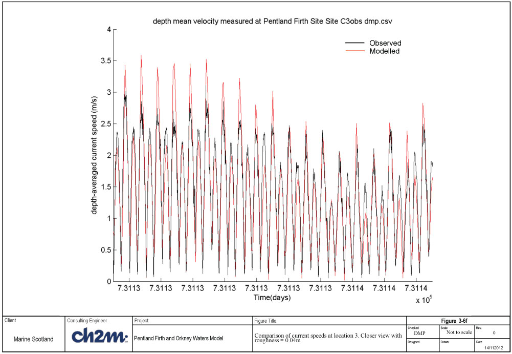
Error statistics have been calculated for depth-averaged current speeds for each of the two roughness sensitivity runs (0.1 and 0.04m); these are presented in Table 3-2. For the error analysis, the time series of the measured data were interpolated to obtain data at the same time intervals as the output from the model simulations..

The statistics presented in Table 3-2 are as follows:-

• meanMeas = mean of the measurement data
• meanModel = mean of the model data
• rmsError = root mean square of the difference between measured and modelled values
• bias = mean of the difference between model result and measured data
• correlationCoef = correlation coefficient
• bias/meanMeas = mean error/mean measurement

Visual inspection of the peak speeds was also considered.

Table 3-2 Error statistics of depth-averaged current speeds (m/s) for roughness sensitivity

Run\location	1	2	3
Roughness length= 0.1m​	maxMeas: 3.22 maxModel: 3.25 meanMeas =1.32 meanModel =1.26 rmsError=0.25 bias=-0.0629 CorrelationCoef =0.94 bias/mean Meas =-0.05	maxMeas: 3.88 maxModel: 3.54 meanMeas =1.96 meanModel =1.79 rmsError =0.31 bias =-0.17 CorrelationCoef =0.97 bias/mean Meas = -0.09	maxMeas: 3.02 maxModel: 3.28 meanMeas =1.5 meanModel =1.3738 rmsError =0.27 bias =-0.11 CorrelationCoef =0.95 ​bias/mean Meas =-0.07
Roughness length= 0.04​	maxMeas: 3.22 maxModel: 3.64 meanMeas =1.32 meanModel=1.34 rmsError=0.29 bias =0.02 CorrelationCoef=0.94 bias/mean Meas =0.01	maxMeas: 3.88 maxModel: 3.79 meanMeas=1.96 meanModel =1.90 rmsError =0.30 bias =-0.06 CorrelationCoef =0.96 bias/mean Meas =-0.03	maxMeas: 3.02 maxModel: 3.59 meanMeas =1.48 meanModel =1.46 rmsError =0.32 bias =-0.03 CorrelationCoef =0.94 bias/mean Meas =-0.02

Table 3-2 is useful in providing quantitative measures of how well the model reproduces the measured data; which in this case is the depth-averaged current speeds at three locations.

Guidance provided in Bartlett (1998) for calibration of water levels and currents speeds is reproduced below:-

• Water levels to within +/- 0.1m
• Speeds to within +/- 0.1m/s
• Direction to within +/- 10 degrees
• Timing of high water to within +/- 15 minutes
• Alternatively some of these could be expressed in percentage terms:-
• Speeds to within +/-10-20% of observed speed
• Levels to within 10% of Spring tidal range or 15% of Neap tidal range

It is accepted that these criteria might be too testing for all regions of the modelled area. A less stringent expectation might thus be that these conditions should be satisfied for 90% of the position/time combinations evaluated.

Given the high peak speeds observed (difficult to obtain within +/- 0.1m/s) our target has been to attain predicted current speeds within 10-20% of observed speeds, and likewise for water levels, to attain prediction within 10% of the Spring tidal range.

The statistics presented in Table 3-2 are useful in determining the relative change between simulations and whether an improvement in the level of fit has been achieved between simulations. The metric "bias/mean" is useful as this gives an overall measure of the proportion of the difference between the predicted and simulated current speeds in relation to the observed values. For the run with a roughness of 0.04m in Table 3-2, it can be seen that in terms of a percentage these are at or below 3% at all three locations, which lies within the ±10%-20% target given above. The bias shows whether the model is over (positive) or under (negative) predicting the observed data. The run with 0.04m has biases (mean of the differences between the model and observed values) for the three locations which are closer to zero, i.e. closer to the observed values, in this case 0.06m/s or less.

Some of the statistics (rms error and correlation coefficient) initially suggest a slightly better match for the simulation with a roughness of 0.1m, however the bias is also a good indication, as is the visual match of the data which suggested the roughness of 0.04m was more appropriate. Similarly the mean model results are closer to the mean observed data with the lower roughness.

Peak speeds are important for in-situ renewable energy current devices and therefore the observed and measured maximum speed is also presented in Table 3-2. The peak speeds were also used as a target; the 0.04m roughness produced peak speeds higher than those observed, however given the fact that the top 11-17m was not measured then the depth-averaged observed values are likely to be under-stated

It was felt that the roughness length of 0.04m provided the best overall fit to the measured depth-averaged current speeds.

3.3.3.2 Comparison of water levels

Following the comparison of the model against measured current speeds, a comparison against measured water levels was made. This had previously been checked for an initial simulation in 2009 and was found to be good using the AMM model for boundary conditions. Observed tide gauge water levels were available at Lerwick (Shetland), Wick (north of Aberdeen) and Buckie on the Moray Firth. Wick and Lerwick tide gauge level data was obtained from the class A tide gauge data held by the National Tide and Sea Level facility. The gauge data at Buckie was obtained from SEPA. Whilst the water level comparisons for 2009 were good, the comparison with the 2001 period showed a defined difference in mean sea level.

This observed difference in mean sea level appears to be due to the boundary conditions derived from the AMM model, an earlier version than the 2009 results. In discussing the concerns with NOC-L, it was made known that mean sea level in this early version of the AMM model was not checked. Therefore in order to proceed with the 2001 boundary conditions a sensitivity test was undertaken by adding a vertical shift to all of the water level boundary nodes. It was found that the current speed through the Pentland Firth was insensitive to the small vertical shifts made due to the large water depths (>50m in general).

Therefore based upon initial statistical analysis of the model results compared with the measured data at Wick (the closest and most complete tide gauge to the Pentland Firth) a number of vertical shifts were considered before concluding that a vertical shift of 0.62m was required to be added to the mean water levels.

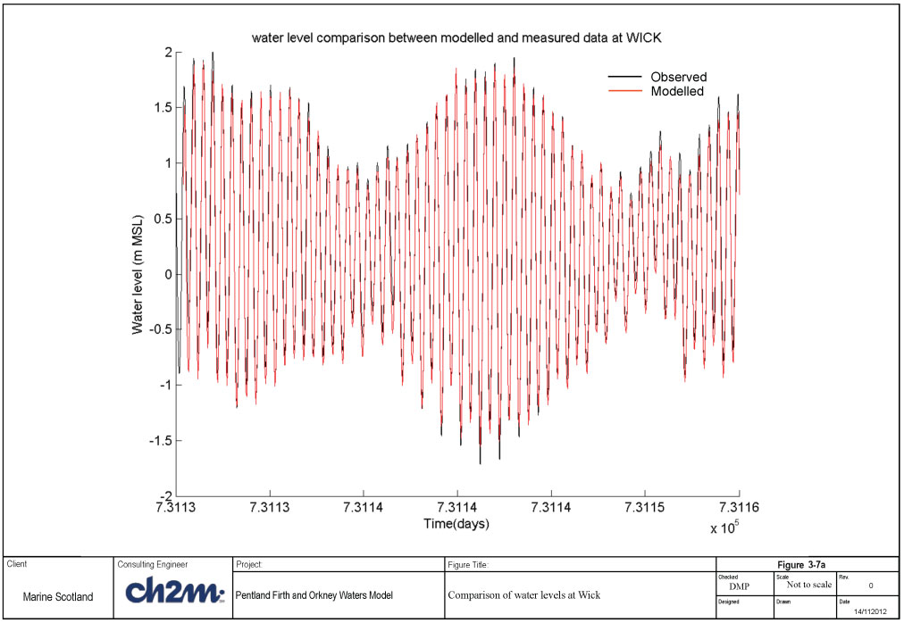
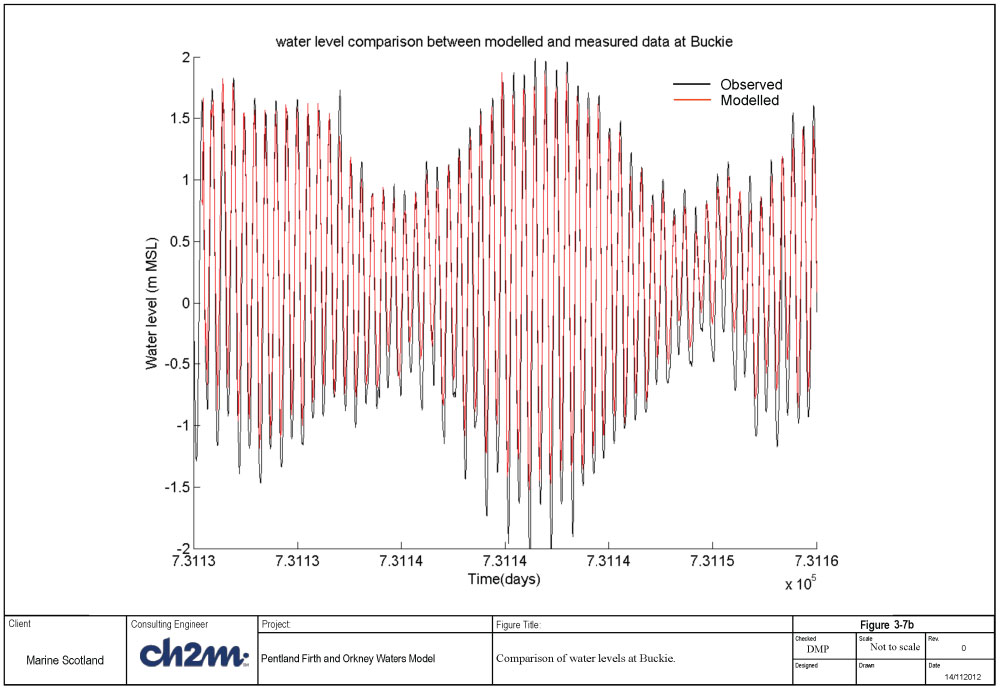
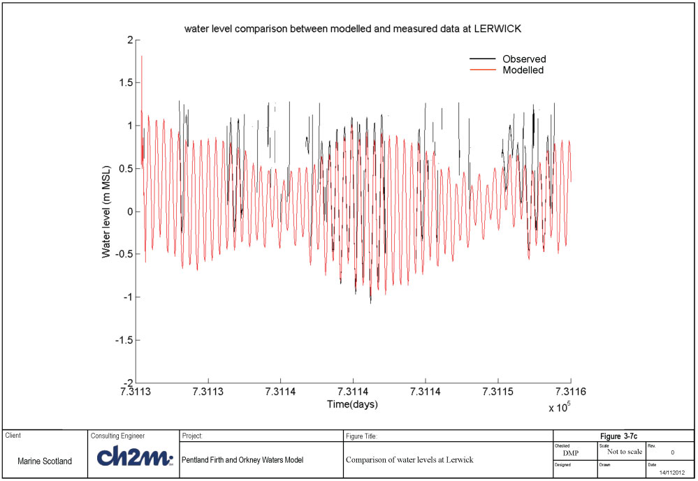
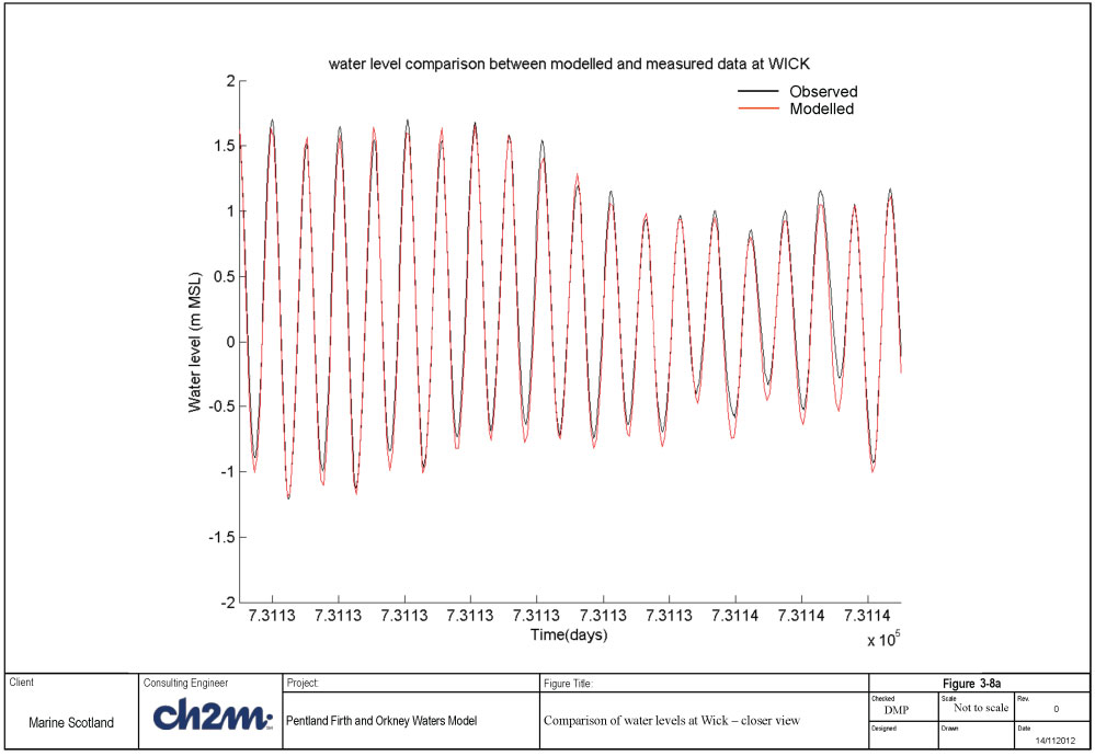
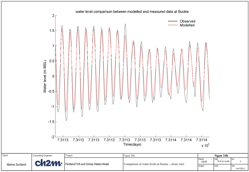
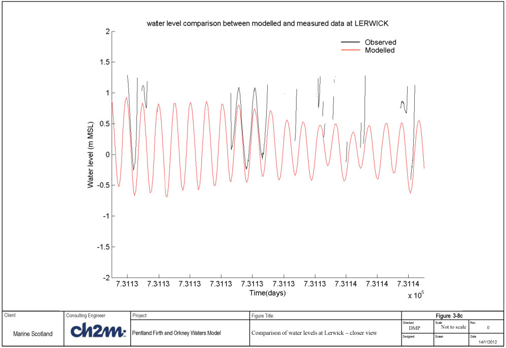
The comparison of water levels predicted by the model compared to the observed tide gauge data can be seen in Figures 3-7a-c as well as a closer view of the same locations in Figures 3-8a-c. The model appears to generally provide a good match especially at Wick. The comparison at Buckie was not quite so good especially towards low water but there was some uncertainty with the datum at this location as well as what appeared to be a two hour timeshift. Comparisons at Lerwick are more difficult in all but a few tides as the tide gauge data quality is not so good which is shown by the erratic nature of the tidal signature.

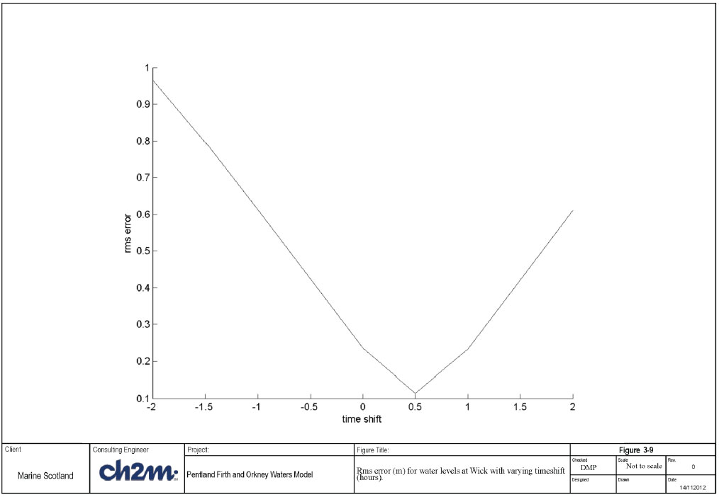
The statistics for the Wick location have been calculated in the same way as for the current speeds. These can be seen in Table 3-3. The middle column provides the statistics for the model, whilst the right hand column provides the statistics for a +0.5 hour phase shift added to the model results. Such an analysis was undertaken to examine if there was a phase shift between the model and observed data. The phase shift analysis is described in the next section 3.3.3.3. The rms error is reduced from 0.23 to 0.11m with the 0.5 hour phase shift. These are all within the guidelines of Bartlett (1998) when considering the magnitude of the rms error compared with the tidal range, then you get a percentage error of 15% (0.23m/1.5m) for the smallest neap tide and 6% (0.23m/3.5m) for the largest spring tide. With the phase shift of 0.5 hours added to the model water level results, these percentage errors drop to 7% and 3% respectively. These are all within the Bartlett (1998) criteria given above.

Table 3-3 summary statistics for WATER LEVELS (m MSL) at WICK

Run\location	WICK	WICK with 0.5 hour shift to model results
Roughness length= 0.04m Vertical boundary datum shift 0.62m (for 2001 only)​	maxMeas = 1.98	maxMeas = 1.98
	maxModel = 1.90	maxModel = 1.90
	minMeas= -1.71	minMeas= -1.71
	minModel= -1.55	minModel= -1.55
	meanMeas = 0.27	meanMeas = 0.27
	meanModel = 0.21	meanModel = 0.21
	rmsError = 0.23	rmsError = 0.11
	bias = -0.05	bias = -0.05
	CorrelationCoef = 0.96	CorrelationCoef = 0.99

3.3.3.3 Phase error analysis

There did appear to be a small phase shift between the model water levels and the observed water levels. The magnitude of the phase shift was investigated by calculating the rms error at Wick for a range of time shifts applied to the model results. The aim was to determine where the minimum rms error occurred and for what time-shift. Figure 3-9 presents the results of this exercise. It can be seen that for the existing phasing the rms error is about 0.23m (for a time-shift of zero). The minimum rms error occurs with a time-shift of +0.5 hours (0.11m).

The rms was calculated for a range of phase shifts for the 3 ADCP locations in the Pentland Firth, there was no phase shift found between the model and the data.

Therefore it appears that the water levels have a phase shift of 0.5 hours whereas the currents do not.

3.3.4 Comparison against transect data

In addition to the timeseries data (at selected locations) that has been used for calibration, a number of transect data sets is also available. These data are available in 2001, 2012 and 2013. The simulations used for comparison are based upon the run with a bed roughness of 0.04m presented above.

3.3.4.1 2001 transect data - Pentland Firth

Transect data was observed during the 2001 survey as presented in Figure 3-4. Figure 3-4 shows the locations of the current stations and the transects which frame the Pentland Firth. This transect data is very useful as it provides a means of determining how the model reproduces the flow through the various entrances/exits to the Pentland Firth.

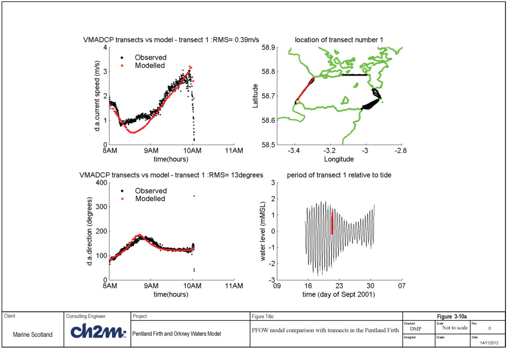
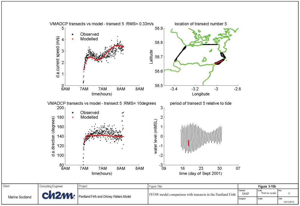
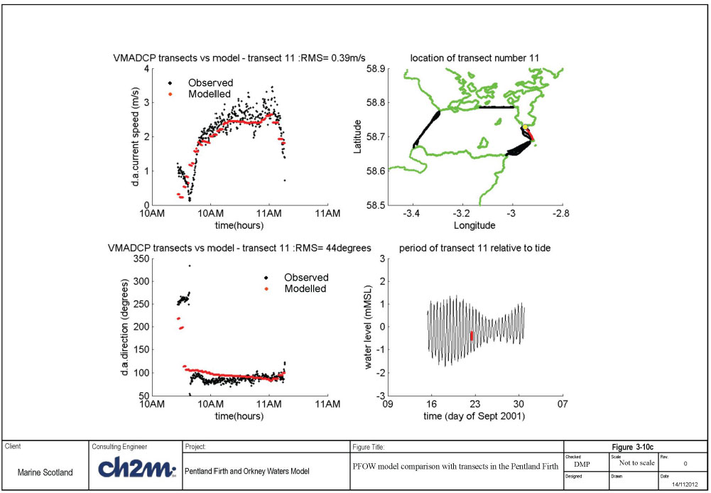
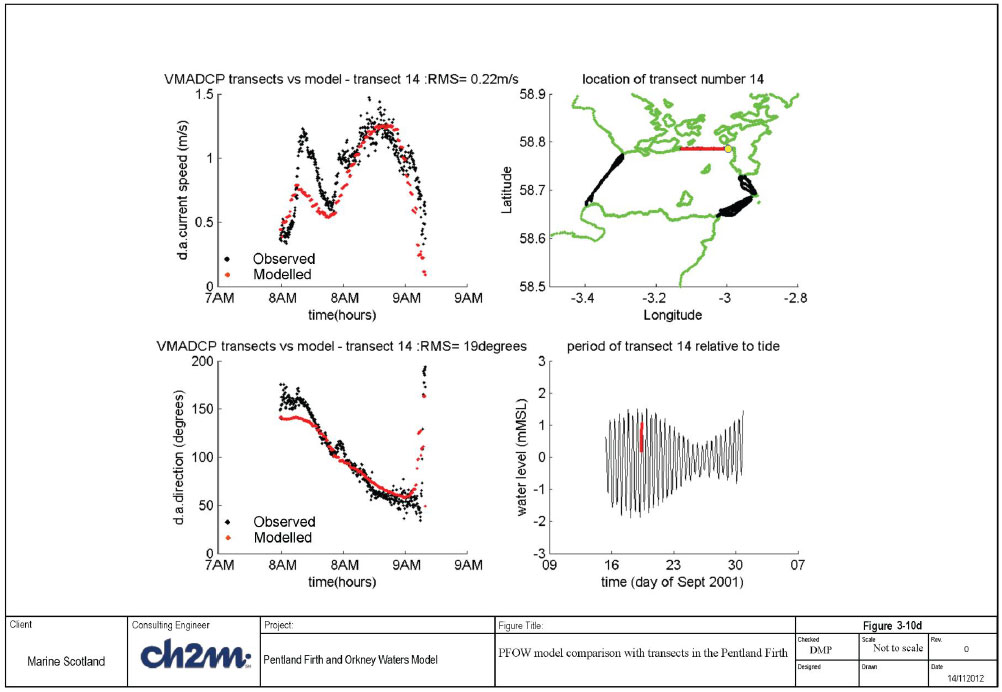
Figures 3-10a-d present the comparison between the observed current speeds (which have been depth-averaged) and the depth-averaged model predictions for the same period in September 2001. Additionally further figures are presented in Appendix B to reduce the number in the main report. Each plot consists of four frames. The top right frame shows the geographic location of all of the transects in black, with the one represented for each figure in red; the yellow dot indicates the start of the transect. The bottom right frame shows the tide curve for the period of the model simulation, with the period of each transect marked in red. The top left frame shows the depth-averaged observed current speed in black, with the predicted current speed in red. Similarly for the current directions in the bottom left frame.

It can be seen in Figures 3-10a-d (and Appendix B, Figures B.1 to B.13) that the current speeds and structure within each transect are reproduced well. The root mean square ( RMS) errors are also provided on each figure. There does appear to be some scatter (variability in the data over short time and space intervals) in the transect data in the order of 0.5m/s. It appears that there are multiple data points at each time however this is due to the scale of the figure and the variation in the recorded magnitude from one measurement to the next. The variation of current speed across each transect is fairly well predicted in the model ( RMS error/Peak speed < 20 to 40%).

3.3.5 2012 transect data - Hoy Channel

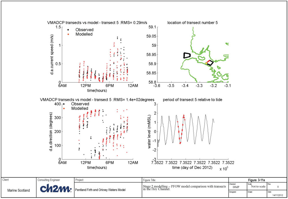
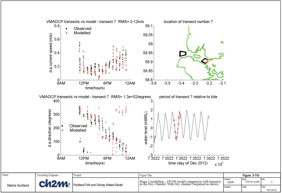
Flow data across a number of transects in the Hoy channel was recorded in December 2012 by Marine Scotland. The model was run for this period to validate the flow model. Figures 3-11 a-b and the Figures in Appendix C (C.1 to C.6) present the comparisons between the observed depth-averaged current speeds across each transect with those predicted by the model.

For this survey two box shapes were traversed throughout a tide by the MV Scotia and transects extracted for each side. Transects 5 and 7 can be seen in Figure 3-11a and b and shows that current speeds are a reasonable match throughout the tide.

The comparisons for transects 1-4 ( Appendix B) are not as good as would be hoped and the reason for this is not known. The comparisons against transects 5-8 are better but still do not provided the level of agreement shown in the comparisons against the transect data in the Pentland Firth. Bathymetry in Scapa Flow is derived predominantly from digitised Admiralty Chart data rather than more recent high density bathymetric data which may be part of the reason.

3.3.6 2013 transect data - Eastern Pentland Firth

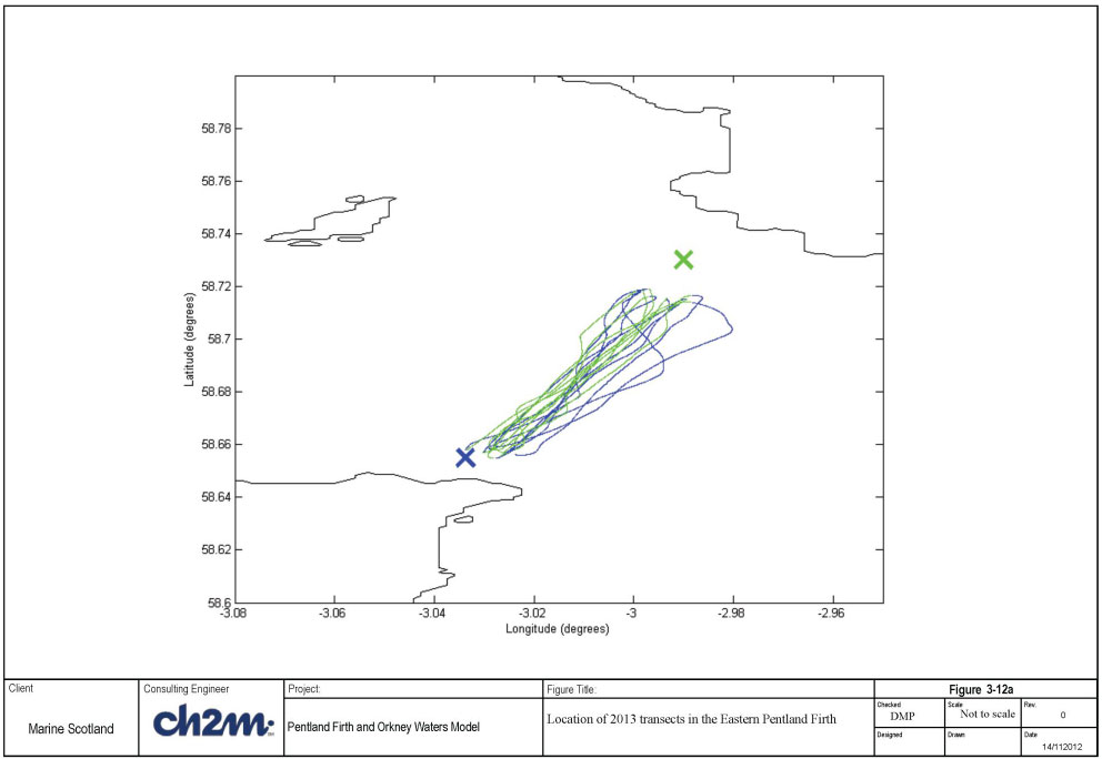
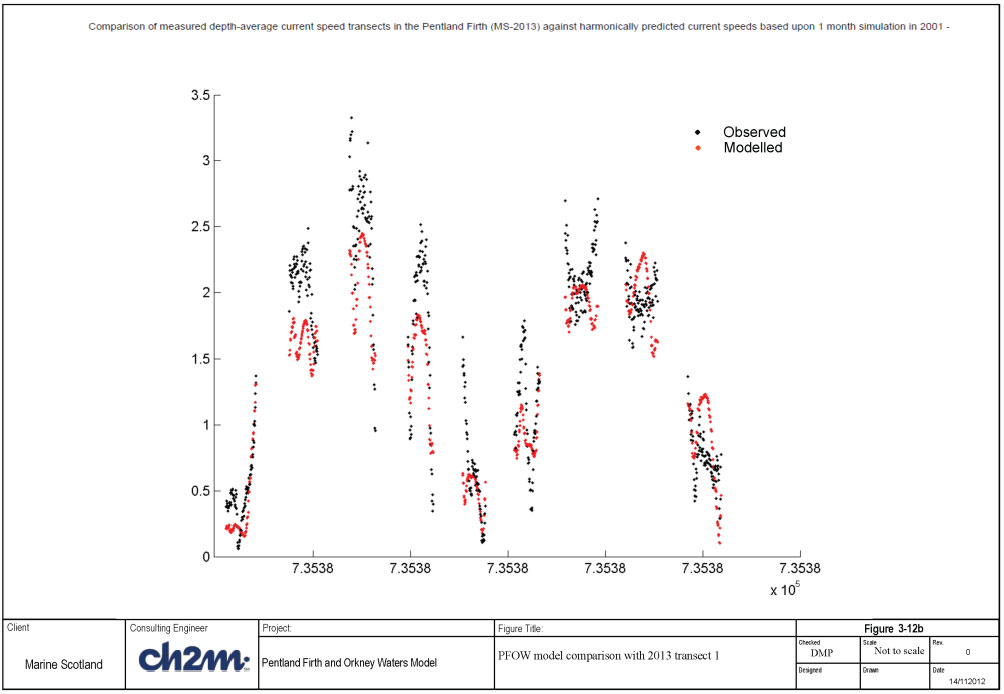
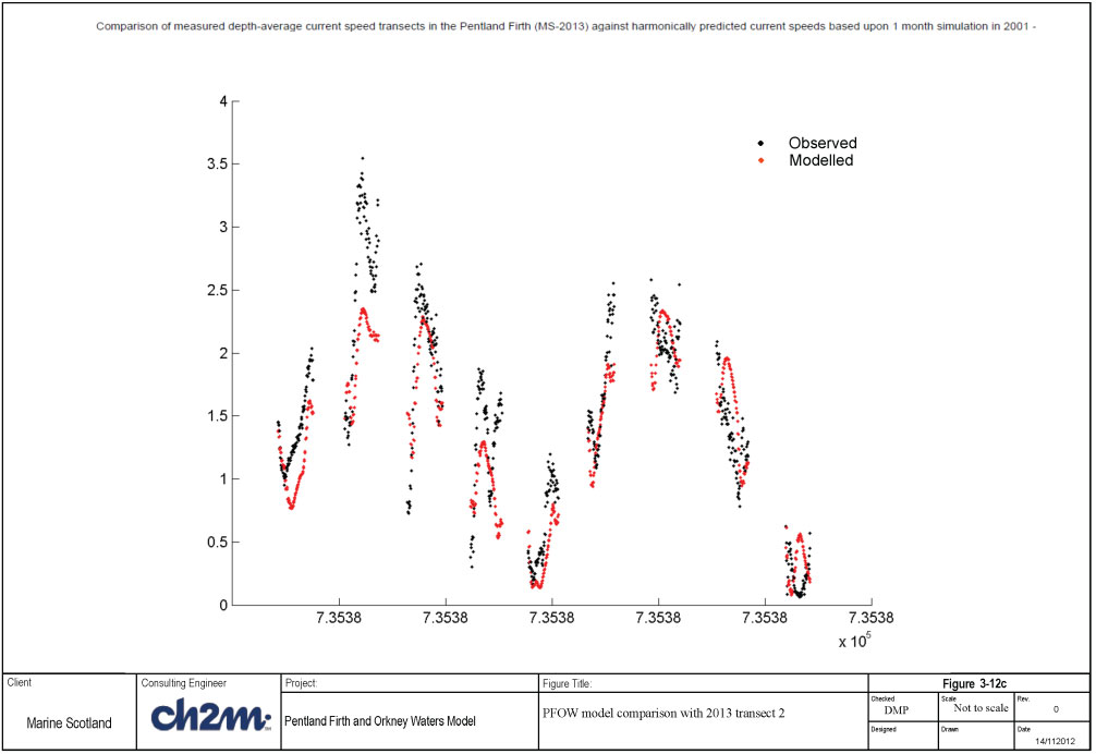
Figure 3-12a shows the locations of transect current observations recorded by Marine Scotland in 2013. One issue in producing the comparison was that boundary conditions from the AMM model were not available and therefore results from the 2001 simulation were used. This was done by first finding the location and time of the observed current speed measurement (depth-averaged), then undertaking a harmonic analysis of the current speed components from the 2001 simulation. Finally the current speed was re-predicted for the period of the survey and the corresponding speed at the time required extracted and plotted. Differences would be expected due to the harmonic analysis and re-prediction process; however it provided a reasonable approach to validate the model in this region.

The comparisons are shown in Figures 3-12 b-c. In general the comparisons are good and reproduce the variation across each traverse. Peak speeds however are under-predicted which may in part be due to the re-prediction of the current speeds from harmonics derived from only one month of model results.

3.3.7 Summary

An FVCOM flow model has been setup for the Pentland Firth and Orkney Waters region. This model has been run in three-dimensions with ten vertical layers and constant temperature and salinity in order to focus on the calibration of the tidal levels and flows. Meteorological forcing, river input and time-varying temperature and salinity have been included in the baroclinic simulations described in Section 3.4.

The measured water level data and current speed data during a 15-day period in October 2001 have been used to calibrate the model. Statistical analysis along with visual inspection of the model results have provided guidance on how to adjust the model parameters (mainly bed roughness and boundary water level datum) in order to improve on the model predictions.

It was found that the boundary conditions extracted from the 2001 AMM model did not appear to be centred on mean sea level when compared against observed water levels. Therefore, it was found that a vertical shift of 0.62m to the water level boundary conditions was required for the model to match the observed water levels more closely.

There also appeared to be a phase error of 0.5 hours in the water level model results compared to the measured data. Analysis of the current data showed that this phase error was not apparent in the current speed results. Data from the AMM model used to create the boundary conditions was provided at one hour intervals. Therefore it is possible that the temporal resolution of this data may in part be attributable to the 0.5 hour phase difference.

Sensitivity tests to bed roughness were performed, which required the default bed roughness to be reduced to a value of 0.04m from the original value of 0.1m. However although locations 1 and 2 compared favourably, location 3 was not as good with higher peak current speeds. This was also observed in the study carried out by Baston and Harris (2011). It should be noted that the observed data was depth-averaged for comparison, although there is no data in the top 11-13m of the water column.

Comparisons of the model results with measurements along transects also show good agreement within the Pentland Firth, but less so in the Hoy Channel.

In conclusion, it is considered that the model has achieved a good level of calibration for the water levels and current speeds compared against the timeseries data. The calibration statistics is within the guidance on water level and current speed calibration provided in Bartlett (1998). Furthermore the agreement between the modelled and the measured current speeds and directions along transects is considered to be satisfactory (by visual inspection).

3.4 Baroclinic model simulations and validation

3.4.1 Introduction

Following on from the calibration of the tidal water levels and currents, the next step in the process of developing the PFOW model is to introduce temperature and salinity boundaries, followed by full meteorological forcing and river inputs and to validate the model against measured data. In this section of the report, the process undertaken to get the model running with the additional forcing and comparison of the model results with observed data is described.

For the purpose of model validation, the period of May 2009 has been chosen as a target period in which to run the model; vertical profile data of temperature and salinity is available during this period within the PFOW model area. The model was originally taken forward as a 3 layer (4 level) model, initially due to run times. There were many stability issues in getting this 3 layer baroclinic model running. These were eventually overcome and the 3 layer baroclinic model was successfully calibrated. However the 3 layer model did not provide the vertical resolution that was felt to be required, especially to enable the reproduction of stratification. The use of the nesting boundaries (see Section 3.2.3) enabled the 10 layer model to run without the stability issues that had earlier been a problem.

3.4.2 Water levels and current speed boundaries

As with the tide-only hydrodynamic model presented in Section 3.3, water level boundary conditions for the baroclinic model have come from the same source; namely the Atlantic Margin Model ( AMM) developed by NOC-L. A water level boundary file was extracted from the hourly AMM-model data for the period June 2009. Additionally as the nesting boundary approach was being used depth-averaged current speeds from the AMM model (vertical variation was not available) were also extracted and applied equally through the vertical for all of the nodes attached to the boundary elements.

3.4.3 Mesh updates

During the process of getting the baroclinic model running, many stability issues were encountered (which were not observed during the tide-only simulations), some of which required adjustments to the mesh. It was brought to our attention that each model node should not be connected to more than 8 adjacent elements. Following inspection of the mesh, it was found to have a number of nodes which had 9 connecting elements. The mesh was adjusted by the addition of extra nodes to remove these features from the mesh. Subsequently the mesh was converted to an SMS format so that the SMS quality checking functionality could be used.

Another issue was with river inputs. If the node at which the river input is applied is connected to two other land boundary nodes in the same element then the water cannot escape from the element and builds up over time to an unrealistic value. A routine was written which moves the location of the river node to the next nearest node.

Bathymetry along the offshore shelf boundary on the western side of the model was also smoothed so that any instability created in this area could be reduced. There were some steep areas which may have caused problems. It is unclear if this alone helped to make the model stable, but it appeared to help prior to using the nested boundary approach.

3.4.4 Temperature and salinity boundaries

As with the water level boundary and nested current boundary, the temperature and salinity nested boundaries have been extracted from the AMM model. Salinity and temperature data is available as daily data over the entire AMM model domain (which encompasses the PFOW model domain). The AMM model has 40 vertical layers with layer numbering starting from the bed. This is in contrast to FVCOM where layer numbering starts at the surface. MATLAB code was written to read in the FVCOM mesh and boundary node locations and extract the relevant data from the AMM model to produce a netcdf format nested boundary file (including the current speed data). Vertical interpolation was employed to provide data at the correct FVCOM level.

3.4.5 Initial conditions

In order to avoid long warm-up periods to get the temperature and salinity to be in dynamic equilibrium, the AMM model results have been used to provide initial conditions for temperature and salinity. First, the hydrodynamic model is run from cold with temperature and salinity applied with constant values. A restart file is then processed using a MATLAB script which interpolates results from the daily AMM model and inserts this data into the restart file overwriting the temperature and salinity data. Then when the PFOW model is started up again using this restart file, not only are the water levels and velocities included (already warmed-up) but so are the temperature and salinity fields.

3.4.6 River input

River data was obtained from CEH (received June 2013 and subsequently updated in August 2014 with data in Shetland waters) and encompassed all of 2009 at 15 minute intervals (Shetland had daily average data). This data was processed using a MATLAB tool which determined which mesh node to apply the river flow to. It also moved the location of a river node to the nearest land node if it was connected to two other land nodes in the same element (if connected in this way, then the river flow cannot escape the element and water levels build up artificially too high).

A river namelist file was produced along with a netcdf file for each of the rivers named in it. On further application of the Shelf model it was found that reading in over 500 river files impacted upon model performance (input/output overhead). The PFOW model was also exhibiting performance issues and therefore all of the rivers (118) were combined into one netcdf file. This, in conjunction with using the latest version 3.1.6 of FVCOM, helped to stabilise runtimes.

The salinity in the river flow was set to 0 psu, and the temperature set to 7 degrees Celsius as this was appropriate for the nearshore temperatures from the AMM model. The river flow is distributed equally amongst all of the vertical layers.

3.4.7 Meteorological forcing

There are two option when including heat input into the FVCOM model; either the net heat flux inputs are provided by way of netcdf files, or FVCOM calculates it internally (from input meteorological parameters). NOC-L found that the shelf model was heating up too much with this approach over a 4-month simulation. Furthermore, they found that this overheating problem was solved by allowing FVCOM to calculate the heat inputs internally. The reason for the overheating problem is due to the difference in sea surface temperature used in the Met Office model and the AMM model used for deriving initial conditions. In the PFOW model the impact is not as obvious as the model boundaries are comparably closer to the middle of the model than for the wide area Shelf Sea model. However it does appear that the PFOW model in its current form using this pre-calculated Met data does produce temperatures which are too high. The boundaries will tend to rectify this but there will be a time lag of a few weeks or more. It is therefore considered advantageous to follow the NOC-L approach and have the heating calculated within the model. This method was adopted in this study.

The meteorological forcing data was retrieved by NOC-L for 2009. This was processed and a Matlab tool produced which provided the necessary meteorological file for FVCOM. A more detailed description of the Meteorological forcing used in both the Shelf Model and the PFOW model can be found in Section 3.2.5 of the report for the Shelf model, Halcrow (2015).

There were some issues with the meteorological forcing data with rain falling on dry elements, some negative evaporation (and precipitation) as well as cooling of elements that were disconnected from the main water body (at a few places along the coastline). Additionally the Met data grid did not always overlap fully the PFOW model. In order to remove issues associated with these problems, the met data was post processed to make the values zero in these locations. It was felt that this would not have a significant impact upon the overall model results.

3.4.8 Stability issues

During the process of obtaining a stable baroclinic model run with all of the met forcing, temperature and salinity boundaries and river inputs, many simulations were performed.

Some of the solutions that were investigated to alleviate model instabilities are highlighted below.

• 9 element connectivity - although the model ran okay for tides only, once this issue was highlighted the mesh was adjusted. This did not appear to solely solve the instability problems, however it was noticed that some instabilities occurred close to a number of these 9 connected nodes, especially close to intertidal areas.
• Sponge nodes - sponge nodes were applied all around the models open boundary. This did provide partial cure to instability issues, however when the model was rerun for the tidal current calibration period, current speeds were lower than previously obtained along with a reduction in tidal range. This was not satisfactory, a range of values were chosen in order to reduce the impact upon water level and speed, however in the end sponge nodes have not been used.
• Roughness - As previously reported during the setup of the model increased roughness around the boundary and specifically higher in the region closest to Aberdeen were applied to the model in order to reduce stability problems and recirculation at the model boundaries.
• Smooth bathymetry at boundaries - For some simulations, instabilities at the model boundaries were observed. It was not always the reason for the model to crash however smoothing the bathymetry did appear to help.
• Deepened river nodes - although this was not observed as a direct cause of instabilities, it was surmised that it may cause a problem if the river flow is being applied to a dry node. The surrounding elements were therefore deepened to 2m below MSL so as to be wet throughout a tidal cycle.
• Timestep - Although the hydrodynamic model with tide forcing only ran successfully with a timestep of 1s, the baroclinic model had stability problems. It appeared that on top of the adjustments made above to reduce instabilities, it was the reduction of the External timestep to 0.75s, and then subsequently to 0.5s which finally produced a model that would run through to a month long-simulation.

Many of the approaches above were investigated due to the problems experienced using only elevation boundaries (no current boundary) and nudging boundaries for temperature and salinity. There was a vast improvement in model stability when the nesting boundary approach was used. The model therefore did not require a spatially varying roughness map but used a constant one in the end. The external timestep did need to be reduced to 0.5 seconds because of the high flows through the Pentland Firth (combined with mesh resolution and depths) although the river nodes did not need to be deepened. The bathymetry was smoothed four times (with coefficient 0.5) using the FVCOM toolbox smoother.

3.4.9 Comparison of tide levels

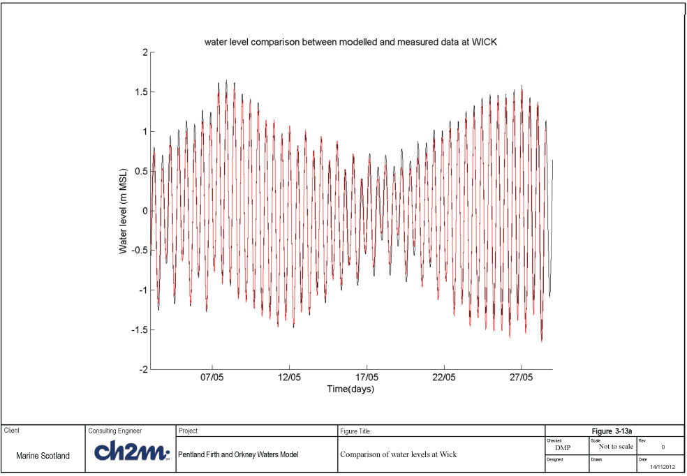
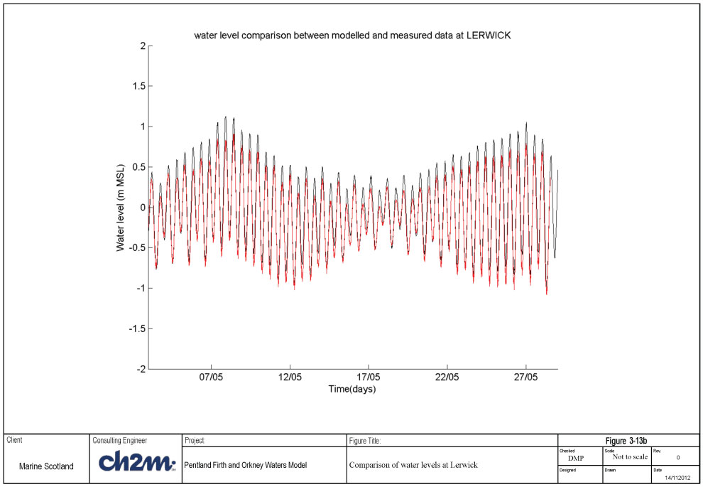
As for the tide-only model, the water levels predicted with the 10-layer baroclinic model have been compared against tide gauge data at Wick (on the mainland, southeast of the Pentland Firth) and Lerwick on Shetland; the comparisons can be seen in Figures 3-13a and 3-13b respectively. Comparisons at Wick are very good, with a good reproduction of the surge around the 7th May 2009, with under-prediction in the order of 0.1-0.15m. There does appear to be some under-prediction of the tidal range during neap tides, but in general during spring tides differences between observed and predicted water levels are within 0.1m. The rms error at Wick for the full month is 0.137m with a bias of less than 3cm. At Lerwick, the prediction of the tide curve is good, however the mean sea level appears to be about 0.1m lower than observed. The rms error is 0.14m with a bias of -0.1m. If the observed water level is lowered by 0.1m (if there is a consistent error with the gauge or model MSL at this location) then the rms error drops below 0.1m.

3.4.10 Comparison of model results against vertical profile data and the AMM model - ten layer baroclinic model, May 2009

This section presents results derived from the 10 layer baroclinic model. Temperature and salinity profile data was obtained from the BODC website ( www.bodc.ac.uk) and filtered for the PFOW model area. This showed that there were a number of locations within the model domain where vertical profiles existed in May 2009. This data provides a means to show how the baroclinic PFOW model performs against temperature and salinity through both the vertical and horizontal planes.

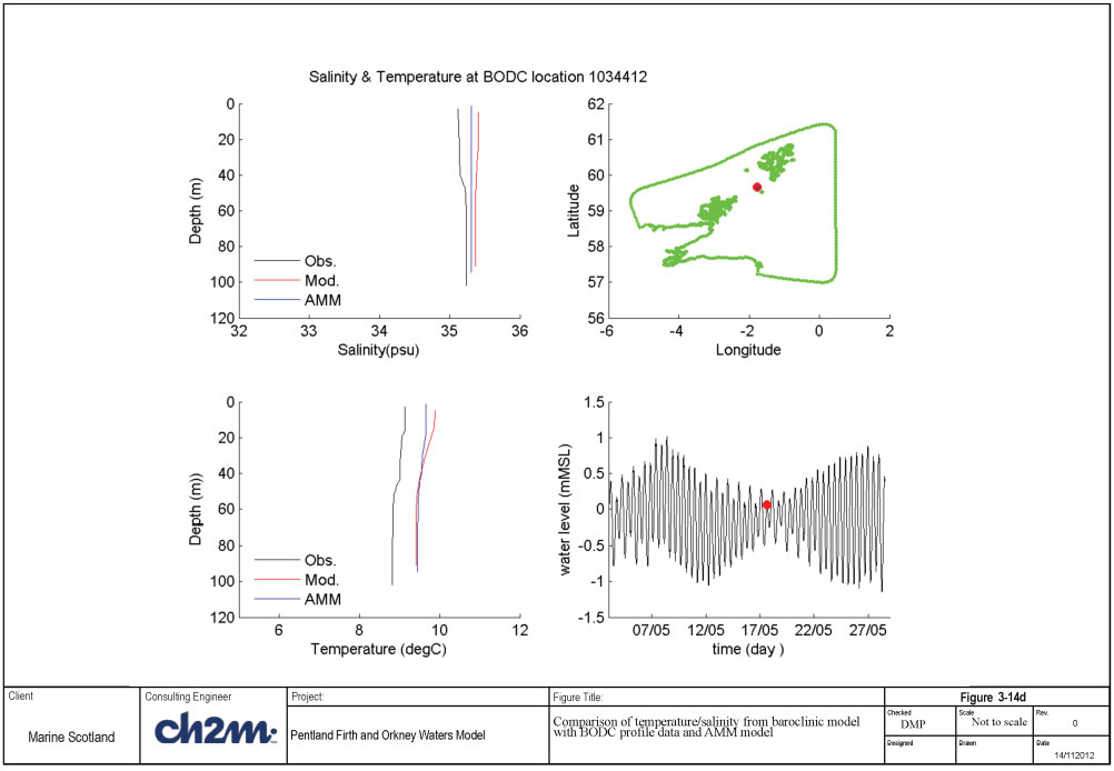
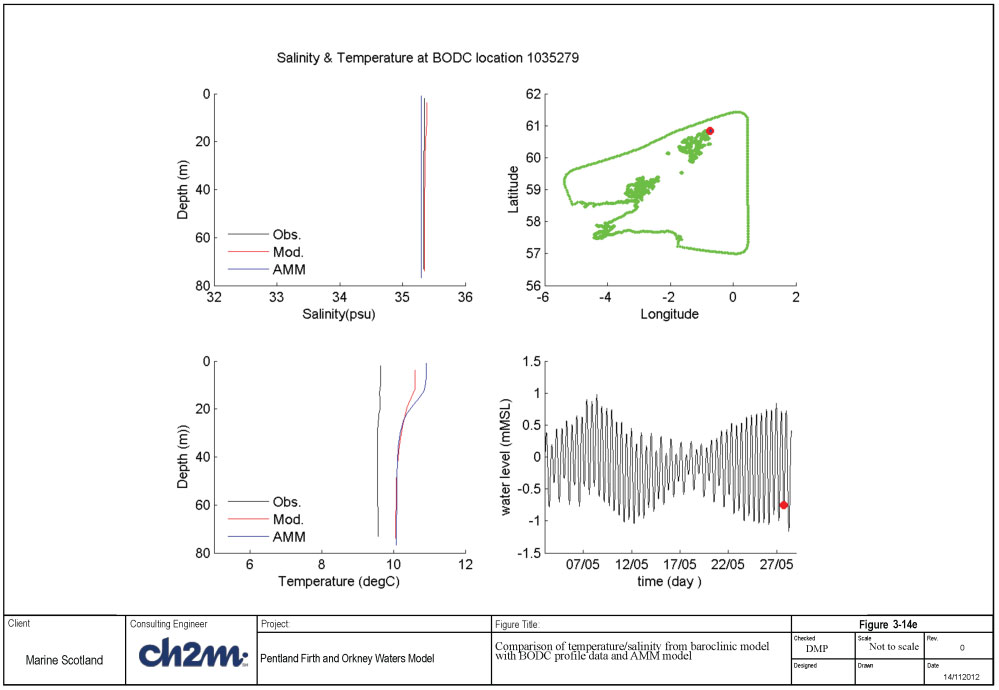
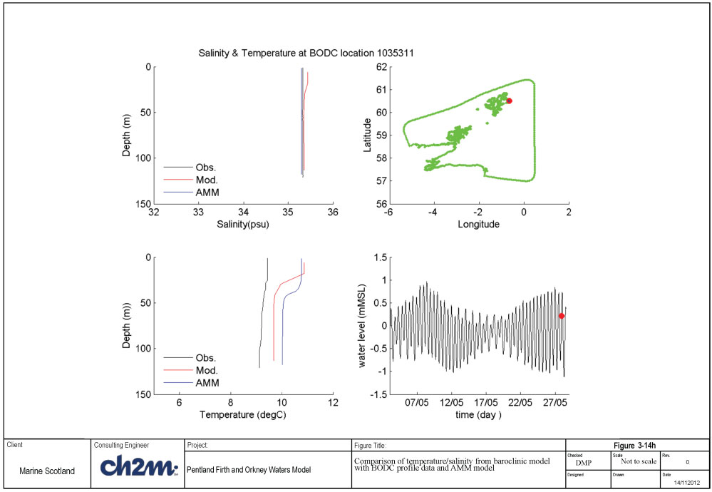
A 20 hour coldstart run was undertaken first so as to build up the water level and flow conditions, and then the hotstart file had the temperature and salinity fields inserted into it from the AMM model. The hotstart simulation was run until the end of May 2009. The results from this simulation have been compared against the available vertical profile data as well as the AMM model results and are presented in Figures 3-14a to i and Appendix Figures D.1 to D.28. Commentary on a few are picked out for discussion below.

Each Figure consists of four subframes. The top right frame shows the location of the measurement; a red circle shows the exact location, and the blue dot shows the nearest model node at which the model results have been extracted. Observations which are slightly outside of the model domain beyond the shelf edge have not been presented. The bottom right frame shows the time at which the profile was taken in relation to the tide curve at that location. The top left frame presents the salinity plotted against water depth (0 being the water surface), and the bottom left frame shows the water temperature against water depth.

The aim has been to get the salinity predictions to be within +/-1psu, and temperature within 0.5 degrees Celsius. Figures 3-14 a-d show comparisons of vertical profiles in between the Orkney and Shetland Isles during periods of neap tides. In general the salinity comparisons are within the target of 1psu, with the largest differences being close to the surface where the effect of fresher water is apparent. As the PFOW model is being driven by boundary conditions from the AMM model there are some limitations as to how close the PFOW model can get to the data, in addition it should be noted that the river flow included in the AMM model is different to that used in the PFOW model which may also account for some differences between the two models. Figures 3-14a and b show similar features to the data in the vertical salinity profile whereas the AMM model is showing no vertical difference. Figures 3-14c and d are located further north than the locations in Figures 3-14a and b, they also do not show quite as good a comparison with the salinity.

The temperature profiles in Figures 3-14 a-d are very similar in shape to those of the observed data, although it can be seen that the underlying temperature is being dominated by that introduced through the boundary from the AMM model. It is therefore not possible to meet the criteria of 0.5 degrees difference between the PFOW model and the observed temperature data given the AMM model results have an underlying over-prediction of 0.5-1 degrees. At these locations in the channel between the Orkney and Shetland Isles, temperatures predicted by the PFOW model are however within 1 degree of the observations.

Figures 3-14e-i show comparisons of temperature and salinity between the models and data in an area around Shetland. In general the comparisons for salinity are very close, although the PFOW model shows slightly higher salinity (order of 0.2 PSU) close to the surface than the data or the AMM model. Figure 3-14i shows a much closer comparison with the data however closer to the surface. The influence of freshwater at this time and location appears to be less than that further to the south. It has been observed in the model results that the influence of freshwater from the west coast of Scotland and the north coast enters the Pentland Firth from the west but also is pushed northwards around the Orkney Isles which is probably why the earlier figures (3-14a-d) showed a larger variation of salinity close to the surface.

Figures 3-14e-i also show the temperature profiles from the PFOW model compared against the data and the AMM model. These locations are closer to the model boundary and therefore a stronger influence from the AMM model could be expected. As previously noted, temperatures are generally over-predicted by the AMM model (in the order of 1 degree Celsius) which has been passed into the PFOW model. The PFOW model however does reasonably reproduce the vertical features in the observed data.

So to conclude, the 10 layer PFOW baroclinic model is able to reproduce salinity within the 1 PSU target. However, the PFOW model has not been able to achieve the 0.5 degree target for temperature but this is thought to be mainly due to the AMM model boundary conditions introducing temperatures which are slightly too high at the model boundary. In general however temperatures predicted by the PFOW model are within 1 degree Celsius of the observed data.

3.4.11 Timeseries comparisons of temperature and salinity

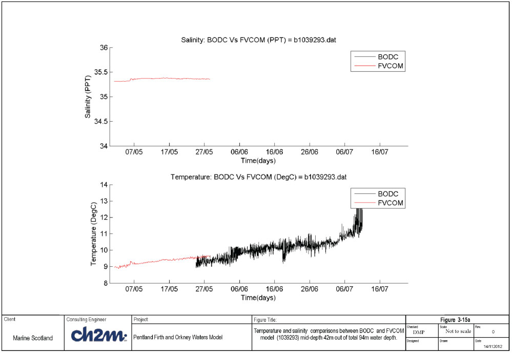
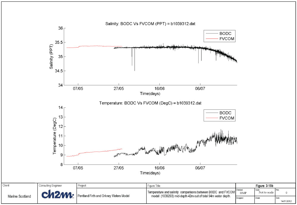
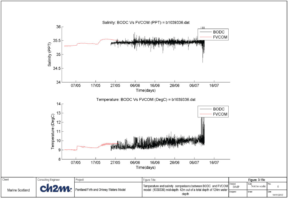
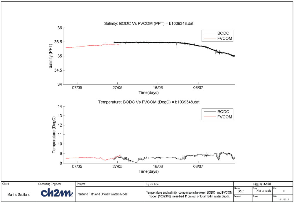
In addition to the vertical profiles, timeseries data of temperature and salinity were available at two locations to the east of the Shetland Isles (obtained from the BODC). Two locations are available, recording at mid-depth and near-bed. There is a short overlap with the results from the simulation in May 2009 which provides a good indication of how the model is performing in relation to variation over time.

The comparisons between the model predictions and the observed data can be seen in Figures 3.14a-d. The model results from the appropriate layer has been presented.

Figure 3-15a shows only temperature comparisons. The build-up of temperature in the mid-depth of the water column appears to be increasing at the same rate as observed with the data and is reproducing the observed temperature within 0.5 degrees Celsius. Figure 3-15b presents the comparisons at the same location but close to the sea-bed. There appears to be less scatter/variation in the temperature measurements with this instrument. Again the model (red line) is approximately 0.5 degrees higher than the temperature observed. This may in part be due to the temperature introduced from the AMM model as discussed in the previous section.

Figures 3-15c and 3-15d present the comparisons of temperature and salinity at the other location at mid and near-bed depths. The mid-depth is at 42m out of a total 124m. Both temperature and salinity have reproduced measurements closely at this depth (salinity within 0.2ppt, temperature within 0.5 degrees Celsius). At the near-bed measurement, the salinity comparison is within 0.2ppt whereas the temperature is very close to that observed.

In general the comparisons have shown the background temperatures and salinities within the model are reproduced fairly well although there are indications that the boundary conditions introduced from the AMM model have increased the PFOW model temperatures by up to one degree Celsius.

3.4.12 Summary

In Section 3.4, the model setup and validation of the baroclinic model has been presented. There were a number of issues relating to model stability that were eventually overcome in order that the 10 layer version of the model could run satisfactorily. The original model setup used a water level boundary only with nudging boundaries for temperature and salinity; velocities at the boundary were derived by the model. With this configuration there were many problems encountered with stability. Eventually after much work trying to improve the stability the move to using nested boundary conditions was undertaken. This approach has provided a much more robust and stable model built upon the earlier work on improving stability. All other Stage 2 models in this study were developed using the nesting boundary approach. The internal calculation of the heat fluxes was also chosen after initial findings from the Stage 1 shelf model. River flow data was updated late in the study with the inclusion of daily river flow data for Shetland (all other river locations include 15 minute data).

Comparisons of the 10 layer baroclinic model against vertical profiles and timeseries have shown a reasonable comparison against the observed data. Salinity is generally within 1 psu in line with our target. Comparisons of temperature however have in general been within 1 degree Celsius but outside the 0.5 degrees Celsius which was our target. Much of this difference however can be attributed to the AMM model boundary conditions (which are also too high) that have been used to impose temperatures at the PFOW model boundary.

3.5 Climatology model simulations

3.5.1 Introduction

The requirement is to produce a one-year climatic run based on climatological forcing, which will represent a typical annual cycle. This was carried out using the Scottish Shelf model climatology results as initial conditions and boundary conditions. The input data sets for climatological meteorological forcing and climatological river fluxes used in the shelf model were also used for the PFOW model. For a full description of the input data, the sources and how it was processed for climatological runs see the Scottish Shelf Modelling report, Halcrow (2015)

The results from the climatic run have been compared with climatological atlas information for temperature, salinity and currents. This provides a distribution of the typical tidal and residual currents over PFOW used as input for particle tracking and to develop connectivity indices in Stage 3.

3.5.2 Boundary conditions

Mean boundary forcing for water levels (mean yearly tides), currents, temperature and salinity were taken from the Scottish Waters Shelf model climatology results. Hourly results were interpolated on to the nested boundary nodes and elements using a Matlab script. Because the shelf model is run with 20 layers while the PFOW model is run with 10 layers it was also necessary to interpolate the current components, temperature and salinity from 20 to 10 layers. This was also carried out in the Matlab script.

3.5.3 River input

River climatology data was processed by NOC-L from G2G river climatology (1962-2011, 577 rivers) provided by CEH. For full details of how the river data was reconstructed to give climatological daily averages see the Scottish Shelf Modelling Report (Wolf et al. 2015).

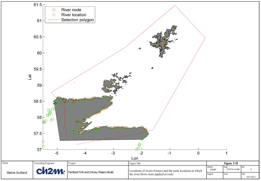
Only 113 of these rivers fall within the PFOW model domain. The rivers were processed in the same way as those for the Baroclinic model runs. Figure 3-16 shows the location of the rivers and the location of the nodes the rivers were applied at.

3.5.4 Meteorological forcing

Met forcing data for the climatological simulations were interpolated on to the PFOW mesh from the Shelf model met forcing input files at 6 hourly intervals. The met forcing was derived by the NOC-L from ECMWF (ERA-40 and ERA-Interim, licence granted). The ERA-interim data cover 1989 - present, and ERA-40 1957 to 2002. These data were processed to derive monthly mean wind-stress, pressures, heating and evaporation minus precipitation for the period 1981-2010, to match the boundary forcing period.

The met forcing were derived as monthly means, which were then linearly interpolated to 6-hourly smoothed forcing data for each grid-point of FVCOM i.e. mean February data were applied at the middle of February; then mean March data were applied mid-March etc., with time-interpolation between. For full details see the Shelf Modelling report, Halcrow (2015)

3.5.5 Temperature and Salinity Comparisons

Average monthly sea surface temperature ( SST) and sea surface salinity ( SSS) observations are available from two sources:

1. The ICES dataset ( http://www.ices.dk/marine-data/data-portals/Pages/ocean.aspx) gridded and averaged for 1960-2004 (45 years) by Jason Holt. Data are also available from the NOAA/ NDBC World Ocean Atlas (2013;
2. The WOA (World Ocean Atlas) http://www.nodc.noaa.gov/OC5/woa13/) based on over 100 years of observations interpolated on to a 0.25° resolution grid.

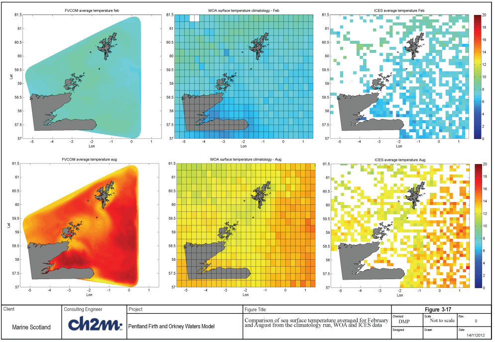
These datasets are used for qualitative comparison with the PFOW FVCOM results for Febuary and August. These months were chosen based on the findings of Berx and Hughes (2009) that the maximum and minimum of the SST occur in February and August.

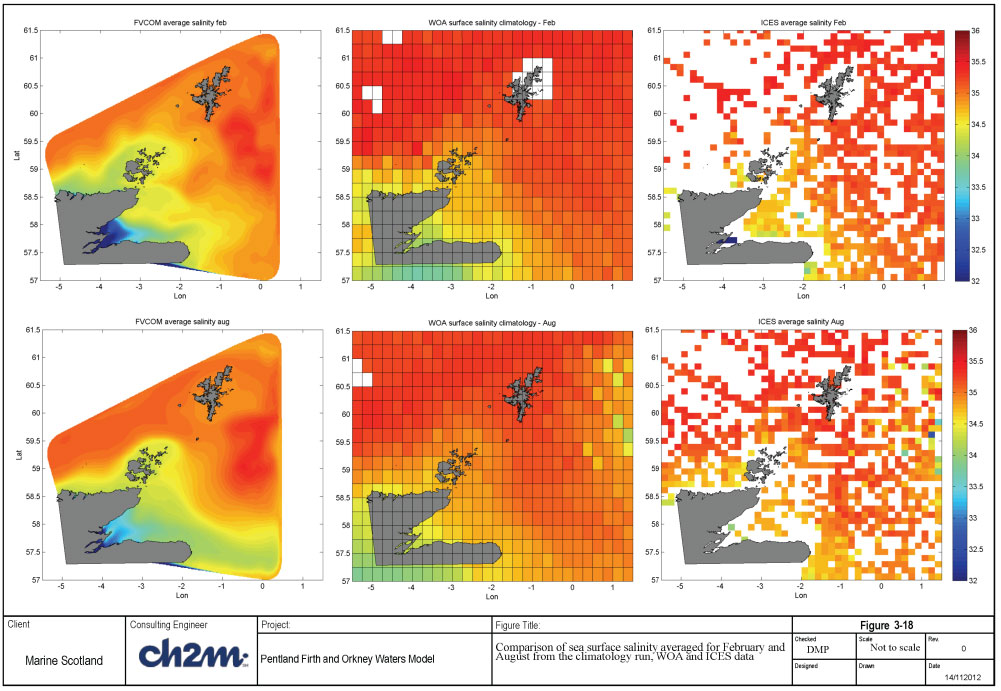
Figure 3-17 shows the comparison of the data sets for SST. The spatial variations in SST, i.e. cooler to the east of Shetland and Orkney in February is not clear in the PFOW FVCOM results. The variation in the August temperatures (i.e. warmer to the east of the islands in August is seen in the PFOW FVCOM results. However, the FVCOM results give slightly higher average SST for February and August, than the WOA or ICES data sets. The PFOW SST are greater that the shelf model temperatures. Figure 3-18 shows the SSS comparison for February and August. The salinity close to land were rivers are discharging are lower in February than August due to the relative levels of rainfall. Compared to the WOA and ICES data sets the FVCOM results give lower salinity levels close to land.

3.5.6 Mean Residual Currents

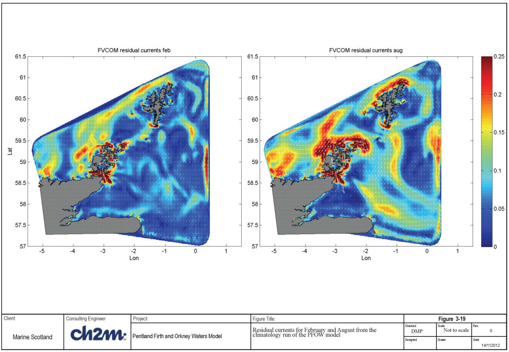
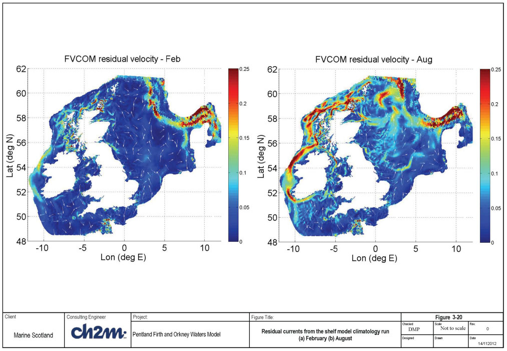
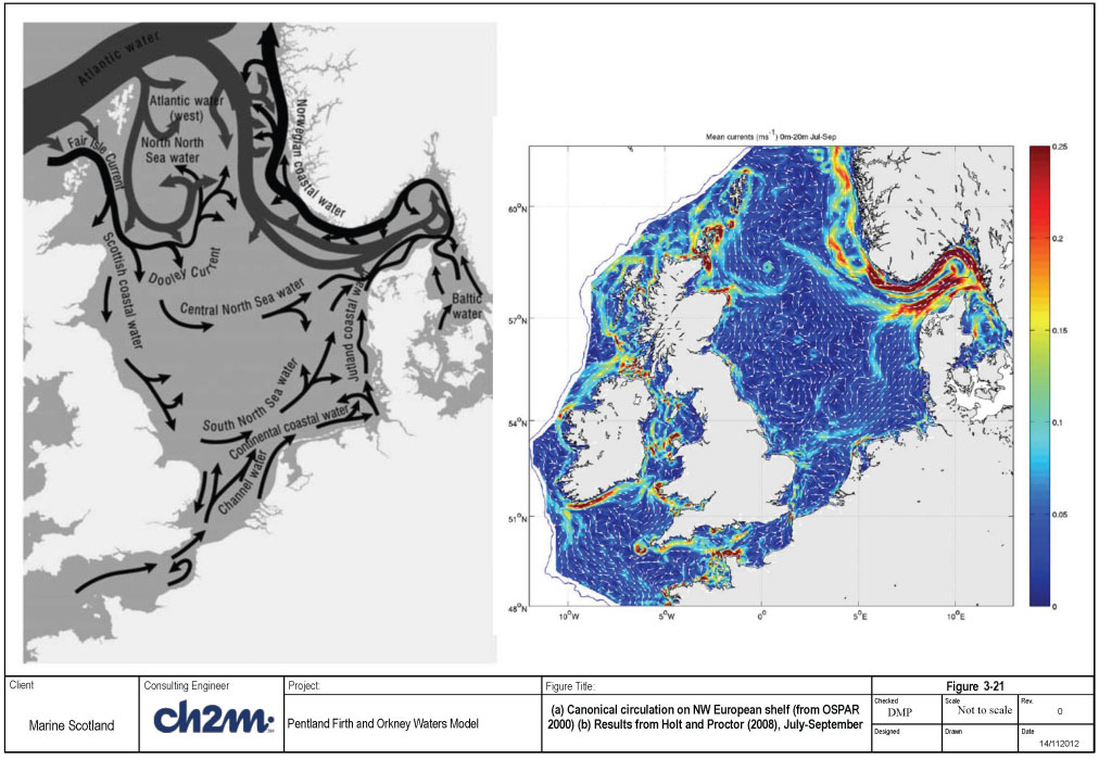
Mean residual currents are shown in Figure 3-19 for February and August. The residual currents from the Shelf model and data from OSPAR (2000) and Holt and Proctor (2008) are presented for comparison in Figure 3-20 and Figure 3-21 respectively. These show general agreement for the magnitude and patterns of the residual circulation.

3.5.7 Summary

Section 3.5 describes the climatology run for the PFOW model. The input data used was taken from the Shelf Model for boundary conditions, CEH for rivers and ECMWF averaged data for the meteorological forcing. The model was run for one year the results have been compared with sea surface temperature and salinity climatological data sets and residual currents for the months of February and August. These results compared well with the available data.