The Scottish Shelf Model. Part 2: Pentland Firth and Orkney Waters Sub-Domain
Part 2 of the hydrodynamic model developed for Scottish waters.
Appendix A: Sensitivity to bed roughness
A.1 Sensitivity to bed roughness using the three-layer PFOW model
Initial model runs (using the 3 layer model) for comparison against the 2001 timeseries data used the default bed roughness of 0.1m and a horizontal mixing Smagorinsky coefficient of 0.2. Current speeds from the model tended to under-predict the peak speeds on the flood tides at Moorings (locations) 1 and 2 - see Figure 3-4 for locations. Sensitivity to bed roughness was therefore undertaken with the aim to improve the comparison with the data. Each model was run for a period of 16 days, with subsequent analysis undertaken for the last 15 days.
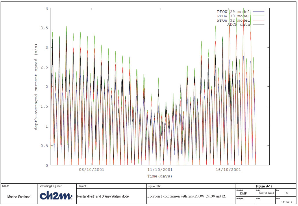
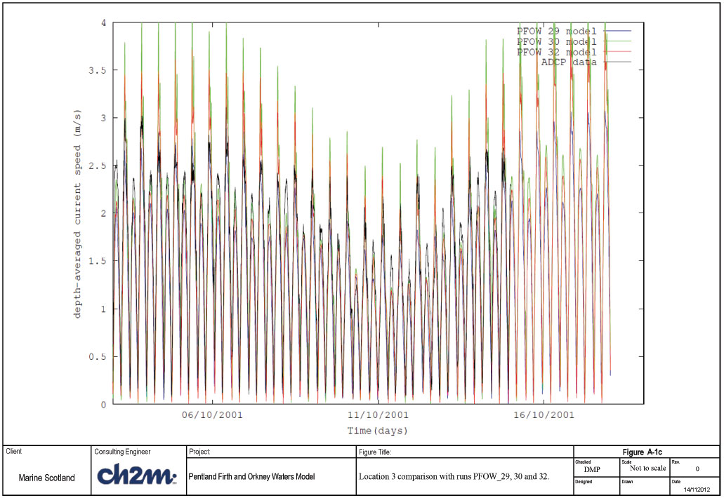
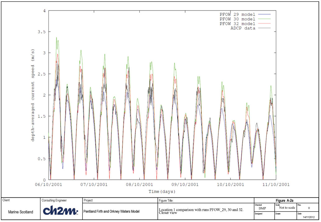
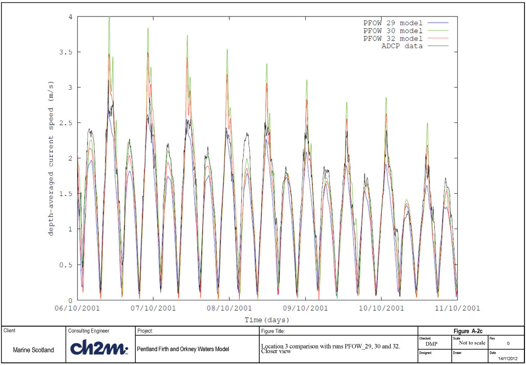
Run PFOW_29 had the roughness length of 0.1m, Run PFOW_30 had a roughness length of 0.01m and run PFOW_32 had a roughness length of 0.025m. The results of the comparison of observed and modelled speeds can be seen in Figures A-1a-c and Figures A-2a-c. Figures A- 2a-c presents the same results but for a shorter time period.
Figure A-1a shows that at location 1 the blue line (PFOW_29 - roughness length 0.1m) appears to under-predict the depth averaged speeds when compared with the measurements. The green line (PFOW_30 - roughness length 0.01m) appears to over-predict the depth-averaged speeds. The red line (Run PFOW_32 - roughness length of 0.025m) appear to bring the predicted depth-averaged peak speeds closer to those observed, with some exceptions. Figure A-2a presents this more clearly. Not every peak is reproduced exactly but the agreement is generally good.
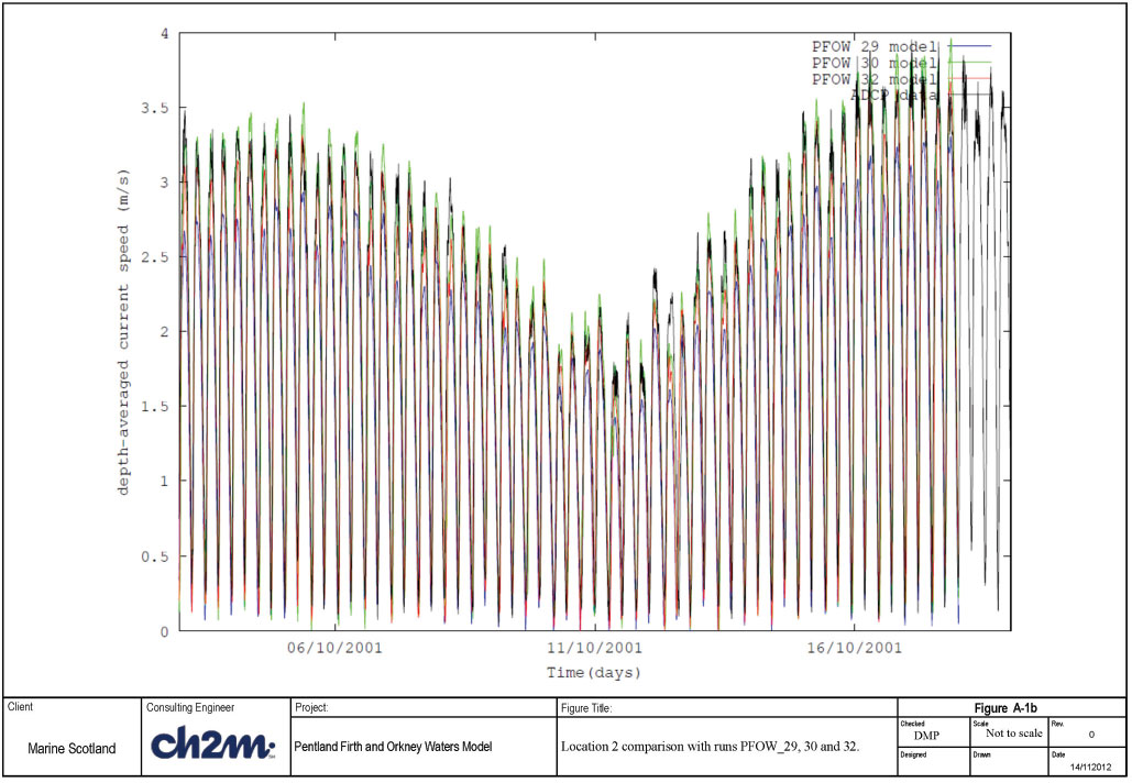
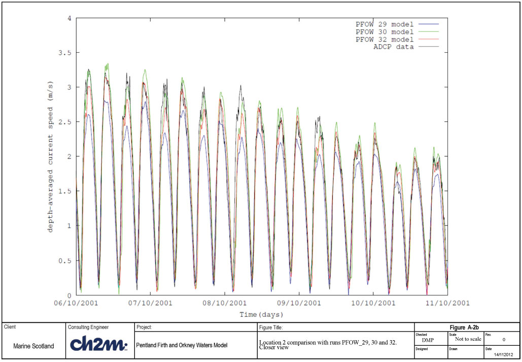
Location 2 results are presented in Figures A-1b and A-2b. It can be seen that again run PFOW_32, with a roughness length of 0.025m appears to reproduce the measurements more closely than the other two simulations. In Figure 3-6b it can be seen that in the first half of the period shown the model appears to be more asymmetric in the flood and ebb speeds, whereas in the latter half the match is better. In general it is felt that visually the PFOW_32 run (roughness length = 0.025m) produces the best overall match.
Location 3 appears to differ from the other two locations in terms of how well the model reproduces the data. At this location the depth-averaged speeds are over-predicted for bed roughness of 0.01m (run PFOW_30) and 0.025m (run PFOW_32). It is the 0.1m roughness length (blue line) which appears to provide a closer match to the depth-averaged currents at this location (see Figures A-1c and A-2c). This suggests that bed roughness should be greater in this area.
Error statistics have been calculated for depth-averaged current speeds for each of the three roughness sensitivity runs (29, 30 and 32); these are presented in A-1. For the error analysis, the time series of the measured data were interpolated to obtain data at the same time intervals as the output from the model simulations.
The statistics presented in Table A-1 are as follows:-
- meanMeas = mean of the measurement data
- meanModel = mean of the model data
- rmsError = root mean square of the difference between measured and modelled values
- bias = mean of the difference between model result and measured data
- correlationCoef = correlation coefficient
- bias/meanMeas = mean error/mean measurement
Visual inspection of the peak speeds was also considered.
TABLE A-1 ERROR STATISTICS OF DEPTH-AVERAGED CURRENT SPEEDS FOR ROUGHNESS SENSITIVITY
| Run\location | 1 | 2 | 3 |
|---|---|---|---|
| PFOW_29 Roughness length= 0.1m |
meanMeas = 1.28 meanModel = 1.13 rmsError = 0.29 bias = -0.15 CorrelationCoef = 0.9 bias/mean Meas = -0.12 |
meanMeas = 1.76 meanModel = 1.50 rmsError = 0.40 bias = -0.25 CorrelationCoef = 0.95 bias/mean Meas = -0.14 |
meanMeas = 1.46 meanModel = 1.22 rmsError = 0.34 bias = -0.24 CorrelationCoef = 0.94 bias/mean Meas = -0.16 |
| PFOW_30 Roughness length= 0.01 |
meanMeas = 1.28 meanModel = 1.33 rmsError = 0.29 bias = 0.049 CorrelationCoef = 0.93 bias/mean Meas =0.04 |
meanMeas = 1.76 meanModel = 1.76 rmsError = 0.29 bias = -0.004 CorrelationCoef = 0.95 bias/mean Meas = -0.002 |
meanMeas = 1.46 meanModel = 1.45 rmsError = 0.33 bias = -0.013 CorrelationCoef = 0.92 bias/mean Meas = -0.01 |
| PFOW_32 Roughness length= 0.025 |
meanMeas = 1.28 meanModel = 1.25 rmsError = 0.25 bias = -0.02 CorrelationCoef = 0.94 bias/mean Meas = -0.02 |
meanMeas = 1.76 meanModel = 1.67 rmsError = 0.28 bias = -0.09 CorrelationCoef = 0.96 bias/mean Meas = -0.05 |
meanMeas = 1.46 meanModel = 1.37 rmsError = 0.28 bias = -0.09 CorrelationCoef = 0.94 bias/mean Meas = -0.06 |
Table 3-2 is useful in providing quantitative measures of how well the model reproduces the measured data; which in this case is the depthaveraged current speeds at three locations. Guidance provided in Bartlett (1998) for calibration of water levels and currents speeds is reproduced below:-
- Water levels to within +/- 0.1m
- Speeds to within +/- 0.1m/s
- Direction to within +/- 10 degrees
- Timing of high water to within +/- 15 minutes
- Alternatively some of these could be expressed in percentage terms:-
- Speeds to within +/-10-20% of observed speed
- Levels to within 10% of Spring tidal range or 15% of Neap tidal range
It is accepted that these criteria might be too testing for all regions of the modelled area. A less stringent expectation might thus be that these conditions should be satisfied for 90% of the position/time combinations evaluated.
Given the high peak speeds observed (difficult to obtain within +/- 0.1m/s) our target has been to attain predicted current speeds within 10- 20% of observed speeds, and likewise for water levels, to attain prediction within 10% of the Spring tidal range.
The statistics presented in A-1 are useful in determining the relative change between simulations and whether an improvement in the level of fit has been achieved between simulations. The metric bias/mean Measurement is useful as this gives an overall measure of the proportion of the difference between the predicted and simulated current speeds in relation to the observed values. For run PFOW_32 in A-1 it can be seen that in terms of a percentage theses are at or below 6% at all three locations, which lies within the 10%-20% target given above.
Peak speeds are important for in-situ renewable energy current devices and therefore on top of the statistics presented above, the closeness of fit to the peak speeds was also used as a target. Analysis of the closeness of fit of the peak speeds is given for a later simulation in this Section.
For the PFOW_29 run, with a roughness length of 0.1m, it can be seen that the bias at each of the 3 locations is between -0.15 and -0.25 m/s. This means that in general the model is under-predicting the current speeds. This is also borne out by seeing that the mean of the model measurements are lower than those of the measurements at all three locations. The rms errors seemed reasonable given the high peak speeds observed although it was felt that there was room for improvements.
Run PFOW_30 had a roughness length of 0.01m. The mean modelled depth-averaged speeds became closer to the mean measured speeds than run PFOW_29, and also the bias reduced to within +/-0.05m/s. Correlation coefficients also improved slightly at locations 1 and 2, but not at 3.
Run PFOW_32, which had a roughness length of 0.025m had the overall effect of reducing the rms error slightly at each of the three locations and increasing the correlation coefficient slightly; both desired effects.
It was felt that the roughness length of 0.025m provided the best overall fit to the measured depth-averaged current speeds. However this work has now been developed further with the use of a 10 layer model.