Developing a methodology to improve soil C stock estimates: report

3. Exploring approaches to improve data used to derive changes in soil carbon stocks

3.1. Geostatistical analysis of the minimum sample numbers required to produce a statistically significant value for total soil C stocks in Scottish peats

3.1.1. Introduction

A geostatistical analysis requires a large number of geo-referenced measurements covering the study region, in this case Scotland. The data are used to inform geostatistical models (variograms) of spatial correlation, which provide estimates of spatial scales of variation. The variogram models can be used to estimate values at unsampled locations and the uncertainty in the estimates. A further application of the technique is to optimise the location of additional sample locations and to estimate how many additional samples are needed to improve the estimates in sparsely sampled areas.

Among the parameters required for C stock estimation, only peat depths were available at a suitable density for geostatistical analysis over Scotland as a whole. Depths were measured in individual peat bogs to characterise peat as a fuel, to aid reinstatement of opencast coal sites and to characterise proposed wind farm sites. The sampled areas were thus determined by factors other than the extents of the peat bogs. Additional information on peat extent over the whole country is provided by the 1:250,000 scale soil map of Scotland (Soil Survey Staff, 1981). The soil map delineates map polygons which provide estimates of the areas occupied by different soils, including the sampled peat bogs. A "peat bog" in this context may be a discrete area of peatland or it may be a named area that forms part of a larger peatland unit. The larger map polygons may include more than one sampled peat bog. The map polygons provide estimates of the areas covered by all soil types in Scotland.

Total C stocks within peatlands are the product of area, depth, bulk density and C concentration. From the available data described above, a suitable unit is chosen for the estimation of these parameters and these are then summed across the whole country. Generally, the unit is the "map polygon" defined by the 1:250,000 scale soil map unit and the component soils are further divided in the vertical plane into soil horizons. The basis of this summation, and the uncertainties associated with each of the components of area, depth, bulk density and C concentration were examined in turn, using all currently available data. It is recognised that the uncertainties in these parameters will vary across the country, and that there is a need for a means of expressing such uncertainty. Essentially, this objective will produce a sensitivity analysis of the parameters that lead to the estimation of peatland C stocks.

Uncertainties in area measurements may be determined by comparing soil map units covering peatland types at the 1:250,000 scale with the greater detail of areas available at larger cartographic scales ( e.g. 1:500, 1:1,250, 1:5,000 and 1:25,000) where these are available for peatland areas. However, the national coverage at 1:25,000 or greater is very restricted, mainly to small lowland bogs. The feasibility of using other databases of peatlands and/or peatland vegetation cover was also examined.

Currently available data on peat depth varies considerably across the country and this has required the estimation of peat depth for polygons where no data exists. Gross C stock calculations were made for different bogs and the whole country by varying depth estimates and assessing the sensitivity of the output.

There is insufficient information on both peatland bulk densities and C concentrations to support any analysis or interpretation of regional variation. Rather, typical bulk densities and C concentrations are, in turn, ascribed to the various peatland types ( i.e. basin peat, deep blanket peat, eroded blanket peat, etc.) and to the specific peat horizons ( i.e. 0-30 cm, 30-100 cm, 100+ cm). Again, the uncertainties in these estimates are determined by varying the C concentration/bulk density used within the calculation and assessing the sensitivity of the predictions to these different input values.

We investigated the feasibility of using spatial statistical methods to enhance and characterize the variation in parameter values, particularly peat depth using available data. The calculation of variance and confidence limits enable estimation of the further sampling required to reduce uncertainties to any chosen level.

In summary, this geostatistical analysis follows a number of steps:

(i) An investigation of how peat depth varies spatially across a peatland area using sites which have been intensively sampled

(ii) A sensitivity analysis which examines the potential uncertainty in depth, area, bulk density and the proportion of C and how they impact C stock estimations

(iii) Utilization of a wider data set on peat depths in order to characterise typical variances and the application to a power analysis

3.1.2. Site descriptions of five typical peat bog areas

Peat depth measurements at many peat bogs were recorded prior to wide availability of computer hardware. Calculation of the mean depths for these bogs was carried out in the ECOSSE project (Smith et al., 2007b). A geostatistical study requires each data point to be captured electronically along with its location (grid reference). The limited availability of computer-stored data sets constrained the geostatistical study of peat bog depth measurements to five sites having detailed peat depth measurements with geographic coordinates. Data in this form were available for three main peatland types:

• lowland basin peat
• semi-confined valley-side peat
• hill (blanket) peat

The five sites with measurements of peat depths were:

• Site A: a lowland peat basin in central Scotland (Coalburn, NS8003400, 1985)
• Site B: valley-side peat in south-central Scotland (Libry Moor, NS710100, 1985)
• Site C: hill peat in north east Scotland (Commercial in confidence, 2003)
• Site D: hill peat in north east Scotland ( ECOSSE project, Glensaugh, NO650800, 2005)
• Site E: hill peat in central Scotland (Commercial in confidence)

3.1.3. Data description

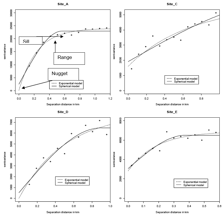
The distributions of sample points on each site are shown in Figure 3.1.1. The data comprise peat depth measurements on either regular grids or along proposed roadways. The original data for one of the sites also included observations where there were no peat layers ( i.e. a peat depth of 0 cm). Since the focus of this study is peat depth, only observations with peat depths greater than zero were included in this analysis. Sites C and E differ from the others as the data points were preferentially sampled, i.e. neither regular grid or random. As described under heteroscedasticity, this is almost certain to have an effect on the sample statistics and an optimal treatment for estimation by geostatistics would involve thinning the points to approximate a regular pattern, although this was not done. The depth measurements on sites A, B and C were measured to the nearest 1 cm by hand augering and examining for mineral material in the auger screw. Measurements on sites C and E were made using a Macintosh probe and recorded to the nearest 10 cm on site C and to the nearest 1 cm on site E.

Figure 3.1.1. Locations of peat depth measurements at five sites (A-E) (scales in kilometres)

Figure 3.1.1.a

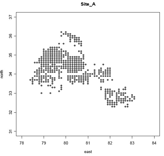
Figure 3.1.1.b

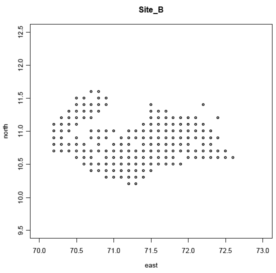
Figure 3.1.1.c

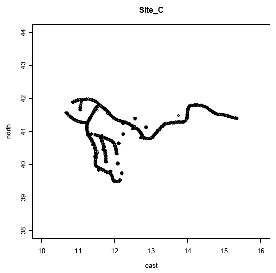
Figure 3.1.1.d

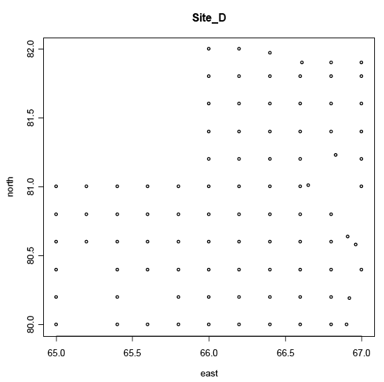
Figure 3.1.1.e

3.1.4. Data analysis methods

An exploratory analysis was done by calculating summary statistics for the five sites, along with histograms and boxplots. These are reported in the following two sections.

Data were analysed using the R statistical package (R Development Core Team, 2008) and libraries for geoR (Ribeiro and Diggle, 2001) and gstat (Pebesma et. al., 1998. Pebesma, 2004).

3.1.5. Exploratory plots

Histograms (Figure 3.1.2) and boxplots (Figure 3.1.3), backed up by normal q-q plots (not shown), of the raw data indicate that transformations are required. In particular, sites A, B and D have long tails of deeper peat. Transformation to natural logarithm or square root would be most appropriate, although this has not been done for the geostatistical analysis, since variograms of transformed data exhibit the same range characteristic. Computing local means and variances in a 1km square, non-overlapping, moving window was done on site A to check if local variability changes over the site. This effect of heteroscedasticity exists for site A where the local variances are directly proportional to the local means (Figure 3.1.4). This is, referred to as the proportional effect (Journel and Huigbregts, 1978) and data having the proportional effect is characteristic for a positive skew. If this proportional effect is present on sites C and E, and areas with low or high values were preferentially sampled, the effect on the variograms would be unpredictable.

The altitudes of the measurements were available for the hill peat sites, but had no effect on peat depths at the scales of investigation.

3.1.6. Descriptive statistics of peat depths

Summary statistics for the peat depths are given in Table 3.1.1. The mean depth of peat on site A, the basin peat site is 123 cm, although the median depth of 48 cm is probably a more accurate estimate of the average depth given there is long tail of depths greater than 100 cm. The valley-side mean depth of 53 cm is also substantially greater than the median of 29 cm. Only one of three hill peat sites, site D, has a median substantially less than the mean. The coefficients of variation were remarkably similar.

Table 3.1.1. Summary of peat depths at five sites (A-E) (cm).

	Site A	Site B	Site C	Site D	Site E
Type of peat	Basin	Valley-side	Hill peat	Hill peat	Hill peat
Number of sites	464	179	943	92	804
Minimum	3	8	10	1	4
1 st Quartile	27	19	40	10	107
Median	48	29	60	30	176
Mean	123	53	71	79	171
3 rd Quartile	178	65	90	135	229
Maximum	630	325	510	300	521
Variance	20962	3261	3453	7125	7119
Coefficient of variation	1.18	1.08	0.83	1.07	0.49

Figure 3.1.2. Histograms of raw data for peat depth for five sites (A-E) (cm)

Figure 3.1.3. Boxplots (after Tukey) of peat depth and log depth at five sites (A-E) (cm). The bold line is the median, the box indicates the inter-quartile range and outliers (indicated by points) lie more than 1.5* IQR (inter-quartile range) away from the upper or lower quartile.

Figure 3.1.4. Site A. Moving (1km square) window variances plotted against means, confirming heteroscedasticity

3.1.7. Statistical tests

Comparing the raw data from the sites with t-tests showed that the differences in the mean peat depths were highly significant at 95% confidence levels for the basin peat compared to the valley side and hill peat. The same was true for the valley side peat compared to the hill peat sites. There was no significant difference between the three hill peat sites. However, since the distributions were skewed with heavy tails, t tests on the raw data should be interpreted with reservation. Computing t-tests with log-transformations of the raw data (Table 3.1.2) indicated that the geometric means were substantially lower than the mean depths computed with the raw data.

Table 3.1.2. Summary of t-test on log-transformed depth data at five sites (A-E) (back-transformed)

	Geometric Mean of Peat Depth (cm)	95% confidence interval
Site A	63.8	57.3 - 71.0 [13.7]
Site B	35.3	31.1 - 40.0 [8.9]
Site C	55.3	52.8 - 57.8 [5]
Site D	32.7	23.7 - 45.0 [21.3]
Site E	143.7	137.1 - 150.6 [13.1]

3.1.8. Geostatistical study

A guide to the number of samples required for robust estimation of variogram models (Webster and Oliver, 1992) indicates that, given certain assumptions, more than 225 data are needed to provide a reliable model The main assumptions are that the variable is normally distributed and isotropic (spatial variation is the same in all directions). This indicates that only site A, site C and site E have adequate numbers of samples for a geostatistical study. The issue of adequate sample numbers is further complicated by the skewed sample distributions on all sites. A further factor is that on site D there appears to be a trend in peat depths from west to east, which could be modelled using a trend function, although this was not attempted given the small sample numbers. Peat depths are thought to vary with external factors, e.g. slope, so a trend model is not unexpected.

Variography

The variogram indicates whether there is spatial dependence in a data set with geographical coordinates. There are three main parameters in a variogram model:

• Nugget - indicating short-range spatial components or measurement errors
• Sill - longer-range spatial components.
• Range - this indicates the spatial scale of correlation between sample points

In the absence of a spatial trend the sill and nugget combined approximate to the overall variance computed by standard statistics.

The spatial dependence can be independent of direction in which case it is isotropic, or dependent on direction - anisotropic. To check for anisotropic spatial dependence, variograms were computed in different directions. Only site C showed anisotropic spatial dependence, related to a trend in peat depths on this site from south to north. Accordingly variograms were computed, pooled for all directions, up to 1 km separation distance (Figure 3.1.5). The plots indicate differences in the spatial dependence on the five sites.

• Site A: depths are spatially correlated up to about 0.5 km
• Site B: no spatial correlation revealed (not studied further since the variogram matches the variance at all separation distances)
• Site C: spatial correlation up to 1 km
• Site D: spatial correlation up to 1 km
• Site E: spatial correlation up to about 0.3 km.

There appear to be differences in the form of the spatial correlation in the basin peat of site A as compared to the hill peat. The basin peat appears to show spatial correlation bounded at around 0.5 km. The hill peat on site C and site D appears to be unbounded up to 1 km distance. The peat depths on site D are greater in the eastern portion of the site so a trend model may be appropriate for these data. Site E appears to show a shorter range of spatial dependence than the other 2 hill peat sites, although this maybe due to an absence of trend here.

Variogram modelling

A weighted least squares approach was used to fit exponential and spherical models to the experimental variograms of peat depth, constrained to a different maximum distance for each site. The model parameters are reported in Table 3.1.3 and the models shown in Figure 3.1.5.

Table 3.1.3. Model parameters for variograms.

	Model	Nugget	Sill	Range (km)	Effective range (km)	Min sum of squares
Site A	Exponential	56	23970	0.238	0.717	5803265
Site A	Spherical	2482	20496	0.567	-	8709780
Site C	Exponential	1604	4052	0.678	2.034	1500671
Site C	Spherical	1912	4001	1.774	-	1579010
Site D	Exponential	0	7851	0.500	1.500	3357099
Site D	Spherical	518	5972	0.901	-	3058862
Site E	Exponential	2832	4062	0.186	0.558	2041525
Site E	Spherical	3067	3427	0.376	-	1997911

Figure 3.1.5 Models fitted for exponential and spherical variograms (no model for Site B due to lack of spatial correlation)

Kriging

Kriging uses the data values and the variogram model to estimate values at unsampled points. When the unsampled points are on a regular grid they produce a map. Computing the variance of estimation or carrying out a simulation using kriging is dependent on a reliable model for the variogram.

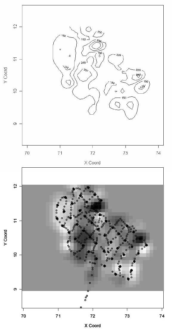
To exemplify the types of maps that can be produced by kriging, ordinary kriging was carried out on the basin peat (site A) and on of the hill peat sites (site E) (Figures 3.1.6 and 3.1.7).

Figure 3.1.6. Contour plot and image plot of ordinary kriging estimates on site A

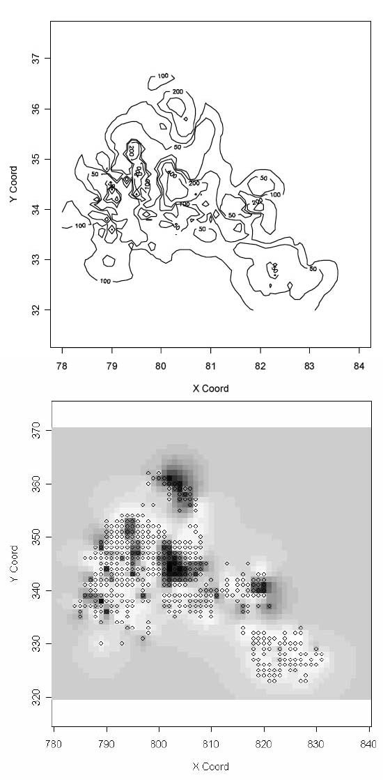
Figure 3.1.7. Contour plot and image of ordinary kriging on Site_E.

3.1.9. Sensitivity analysis on current carbon stock estimates

The ECOSSE project (Smith et al., 2007b) made some new calculations of the stock of C within Scotland's organic soils with particular emphasis on estimating the C stock below 100 cm in the soil profile by incorporating previously unused data on peat depth. While uncertainties in the estimates were acknowledged, a more precise quantification of the errors was not made. A set of analyses has now examined the variance associated with the component elements making up the current C stock estimate for peatlands. These parameters are depth, % C, bulk density and area with the total C stock being the product of all four, i.e.

Total C stock = area x depth x bulk density x %C

Usually %C is measured by analysis of the soil fine fraction ( i.e. a sieved fraction) so a correction needs to applied for the proportion of stones removed. Since we are here concerned with peat the occurrence of stones is generally low or absent. Any large roots may also be removed by sieving so a correction may be required for these. It is a moot point whether roots, living or dead, are included. Logically, dead roots form part of the soil organic matter and are hence part of the peat while living roots are still part of the plant biomass, which is a separate entity; the practical difficulty is distinguishing the two. Inevitably, many fine roots will be included with the soil organic matter.

Since the total stock is a simple product, all parameters contribute equally to uncertainty. However the errors associated with each vary. Also there is variation between them in number of samples upon which they are based and in their spatial location. Each parameter has been examined in turn as to its origin or component data and estimates have been made of their respective standard errors or variances. The summation of variance was determined using simple error propagation equations, i.e. the combined variance is the sum of the component variances. Since the components were all in different units, relative standard errors had to be determined first.

Peatland Area

Estimating the error on the areas of peatland presented a special problem as these areas are on a map and not replicated in any sense. The irregular boundary on a soil map that encloses soil of a particular type, as determined by the soil surveyor, is denoted as a 'polygon', though in practice the term refers to the whole area thus enclosed. While some parts of Scotland are mapped at finer scales, coverage of the whole country has only been made at the 1:250,000 or one to quarter-million ( QM) scale. Polygons on the QM map would be drawn based on survey data and notes in conjunction with aerial photography interpretation. The location of the polygons on the digitised QM map had been digitised using an automated laser light based system and hence unlikely to deviate much from the original QM map. The major error here was assumed to be in the delineation of a particular area on the ground at the time of survey. As a first approximation, the polygons were taken to be circular and the radius not to vary by more than 10% or by 250 m, whichever was less. The area was recalculated on this basis and this was taken to be the 95% confidence interval. Taking the additional assumption that there was no consistent error in determining the polygon boundary, assuming a normal distribution of possible errors and using a Monte Carlo simulation, overall errors on the peatland areas were estimated. These, together with the mean areas are given in Table 3.1.4.

Table 3.1.4 Mean Peatland areas used in the C stock calculations. Data shows means and estimated standard errors (S.E.).

	Area (km 2)
	Mean	S.E.
QM UNITS
Basin Peat	54	8
Semi-confined Peat	5423	360
Blanket Peat	4155	261
PEAT POLYGONS
Basin Peat	673	6
Blanket Peat	3711	24
Eroded Basin Peat	8	1
Deep Blanket Peat	1679	16
Eroded Deep Blanket Peat	309	7
Eroded Blanket Peat	1259	14
TOTAL	17269

Table 3.1.5 Variability in the area-weighted mean peat depth values used in the calculation of C stocks. Data shows means, standard errors (S.E.) and number of values (N).

	Depth (cm)
	All data, measured + judged			Measured data only
	Mean	S.E.	N	Mean	S.E.	N
QM UNITS
Basin Peat	287	34	8
Semi-confined Peat	128	9	71
Blanket Peat	112	7	48
PEAT POLYGONS
Basin Peat	287	9	360	326	29	63
Blanket Peat	134	10	652	220	55	31
Eroded Basin Peat	272	39	4
Deep Blanket Peat	230	15	166	253	43	19
Eroded Deep Blanket Peat	170	4	30
Eroded Blanket Peat	132	8	116	173	54	4
All Peat types				241	44	117

Peat Depth

Estimating the error in the peat depth estimates is complicated by the fact that the peat depth values used in the final calculation were area-weighted averages rather than straight averages. This is necessary as the values are subsequently multiplied by the respective peat areas to give, effectively, a total peat volume. The variance in depth was calculated using the relationship:

Var (?w _i.x _i) = ?w _i². Var (x _i), where x _i is the depth and w _i = area of polygon i/total area.

The means and standard errors for depth given in Table 3.1.5 were calculated from all the peat depth estimates, both actual values and those assigned to areas without measured values by expert judgement. Including all values was judged appropriate since these are the actual depth values used in the C stock calculations. Note that the depths of 287 cm for basin peat in both the QM units and in the peat polygons are coincidental. In three cases, the number of values on which the peat depth is based was quite low; however, these were also categories that occupied the smallest areas, viz. basin peat in the QM units, eroded basin peat and eroded deep blanket peat.

Table 3.1.5 also gives the peat depths returned using actual measured values. Note that there were no data for eroded basin peat or for eroded deep blanket peat though these two types covered the smallest areas. Also there were no measured data for any of the QM units. This is particularly critical as the QM units accounted for 56% of the total peatland area (Table 3.1.4) and 45% of the final C stock (Table 3.1.9). Hence the depth values for the QM units assigned in Table 3.1.5 are based solely upon expert judgement (although the judgement process did include recognition of a few scattered depths recorded in these areas in the survey reports). While this approach is not ideal, it is all that can be done in the absence of measured data; the broad agreement between the expert judgement and values obtained by kriging (see below, figure 3.2.5) give some confidence in the process used. There is clearly a trend for the peat depths including expert judgement to be less than those based on measured values. This is particularly so for blanket peat, which has been reduced from 2.20 m to 1.34 m. An explanation is given in that the measured data were biased towards the 'major peat deposits' with inherently greater depths while the country-wide value includes many peat deposits that are shallower for topological reasons.

Dry Bulk Density

This parameter was originally estimated using a pedotransfer function ( PTF) which relates bulk density to %C. This function was based upon an analysis of 39 data pairs (See Smith et al., 2007b, appendix 1). However, further inspection of this relationship suggested that for peatland samples the relationship breaks down and that the positive regression originally obtained was based solely upon the inclusion of samples from organo-mineral soils, which contained varying additions of mineral material. Hence the dry bulk density values used (Table 3.1.6) were a compilation of the currently available data:

i) Samples taken from Red Moss (Netherley) and Middlemuir bogs as part of the project.

ii) Peat samples used in the original PTF calibration but removing those from organo-mineral soils.

iii) Peat samples from the NSIS_2 phases 1 and 2.

iv) Samples taken from Glensaugh as part of the ECOSSE project (Smith et al., 2007b). As the original dataset contained 145 values, to avoid over biasing this site these were consolidated by calculating mean values for each depth measured of the 3 one km ² squares surveyed, giving 9 values.

In total, 104 bulk density values were obtained. Samples were stratified as being either basin or blanket peat and by depth at 0-30 cm, 30-100 cm and 100+ cm. Further division was not justified as sample numbers were already low in some categories or because further details ( i.e. deep or eroded) were not known. Analysis on the data showed a difference between the mean for all basin peats (0.112 g cm ^-3) and that for blanket peats (0.129 g cm ^-3), which just failed to be statistically significant (P=0.054). There was no significant difference between 0-30 cm (0.134 g cm ^-3), 30-100 cm (0.120 g cm ^-3) and 100+ cm (0.109 g cm ^-3). The greater bulk density values for 0-30 cm possibly reflects a tendency for these surface peats to dry out and compact; this was particularly clear at Glensaugh where samples with high bulk density were also low in moisture content. There was no significant interaction between peat type and depth. The samples were somewhat biased towards the north-east of Scotland with half coming from this region. In particular, there was a paucity of values from deeper peat horizons.

A summary of the bulk density data is given in Table 3.1.6. The value for basin peat was also applied to the eroded basin peat category and the value for blanket peat similarly applied to the other blanket peat categories. There were no independent values for the QM units and so peat polygon values were also ascribed to the respective peat types.

Table 3.1.6 Mean Bulk density values used in the C stock calculations. Data shows means, standard errors (S.E.) and number of values (N).

	Bulk Density (g cm -3)
	0-30 cm			30-100 cm			100+ cm
	Mean	S.E.	N	Mean	S.E.	N	Mean	S.E.	N
QM UNITS
Basin Peat	0.136	0.076	12	0.114	0.068	17	0.092	0.016	16
Semi-confined Peat	0.136	0.076	12	0.114	0.068	17	0.092	0.016	16
Blanket Peat	0.134	0.036	17	0.123	0.023	34	0.143	0.029	8
PEAT POLYGONS
Basin Peat	0.136	0.076	12	0.114	0.068	17	0.092	0.016	16
Blanket Peat	0.134	0.036	17	0.123	0.023	34	0.143	0.029	8
Eroded Basin Peat	0.136	0.076	12	0.114	0.068	17	0.092	0.016	16
Deep Blanket Peat	0.134	0.036	17	0.123	0.023	34	0.143	0.029	8
Eroded Deep Blanket Peat	0.134	0.036	17	0.123	0.023	34	0.143	0.029	8
Eroded Blanket Peat	0.134	0.036	17	0.123	0.023	34	0.143	0.029	8

Table 3.1.7 Mean %Carbon values used in the C stock calculations. Data shows means, standard errors (S.E.) and number of values (N).

	Carbon (%)
	0-30 cm			30-100 cm			100+ cm
	Mean	S.E.	N	Mean	S.E.	N	Mean	S.E.	N
QM UNITS
Basin Peat	51.1	1.0	25	48.6	1.1	43	60.8	3.4	2
Semi-confined Peat	51.1	1.0	25	48.6	1.1	43	60.8	3.4	2
Blanket Peat	50.6	1.8	21	52.9	0.7	49	54.6	3.2	7
PEAT POLYGONS
Basin Peat	51.1	1.0	25	48.6	1.1	43	60.8	3.4	2
Blanket Peat	50.6	1.8	21	52.9	0.7	49	54.6	3.2	7
Eroded Basin Peat	51.1	1.0	25	48.6	1.1	43	60.8	3.4	2
Deep Blanket Peat	50.6	1.8	21	52.9	0.7	49	54.6	3.2	7
Eroded Deep Blanket Peat	50.1	3.5	10	57.1	0.4	8	54.2	1.2	2
Eroded Blanket Peat	53.0	0.9	40	55.2	1.0	33	54.0	3.2	9

Carbon content (%C)

Values for %C in peat were re-extracted from the Scottish soils analytical database in order to calculate the standard errors associated with the values as used. In total 240 values were used. These data are given in Table 3.1.7 with %C values for the three peat layers 0-30 cm, 30-100 cm and 100+ cm. The values were originally obtained from data for basin peat, deep blanket peat, eroded deep blanket peat and eroded blanket peat. Values for blanket peat were taken to be as for deep blanket peat (blanket peat in fact may include deep blanket peat as these areas are undifferentiated). Similarly, eroded basin peat was assumed to be the same as basin peat. For the QM units, where there were no data, basin and blanket peat was taken to be the same as their counterpart polygon values and semi-confined peat was taken to be the same as basin peat. It should be noted that there is a limited database of %C values and particularly so for the peat profiles below 100 cm. Clearly this is not ideal though, in some mitigation, there is a limited range of values of %C for peat, which tend to cluster around 52%.

Relative uncertainties

Table 3.1.8 Basis of parameter estimates used in the calculation of total C stock and their relative errors

Parameter	No. samples	Location	% Error in estimates
Depth	~6000	Country-wide but some areas under-represented	7.2
% C	240	Country-wide but mainly surface (0 - 100 cm)	3.4
Bulk density	104	Country-wide but weighted towards NE Scotland and few deep samples (>200cm)	8.3
Area	1455 polygons	Country-wide	4.5

A summary of the relative uncertainties are given in Table 3.1.8. The %error in the estimates is the mean standard error as a percentage of the mean. Bulk density has the greatest uncertainty among the parameters, followed closely by depth, despite being based on the largest number of samplings. The number of samples for depth is an estimate based upon a limited recount: out of the total of 117 peat bogs with measured depths, 77 totalled nearly 4000 individual depthings (see section 3.1.10). These error values should be treated as being on the conservative side since they hide the fact that the underlying data is not randomly located but biased both in terms of position within the country as well as vertical position in the peat profile. The assumption is that the values currently obtained can be applied to other geographical regions and to other peat depths.

Peatland C stock

Table 3.1.9 Total peatland carbon stocks, means and standard errors, based upon error propagation of component parameters.

	C stock (Mt C)
	0-100 cm		100+ cm		Profile
	Mean	S.E.	Mean	S.E.	Mean	S.E.
QM UNITS
Basin Peat	3.2	0.5	5.6	1.4	8.8	1.5
Semi-confined Peat	323.3	39.3	84.8	28.5	408.1	48.5
Blanket Peat	273.6	15.9	38.8	23.0	312.4	28.0
PEAT POLYGONS
Basin Peat	40.1	4.5	70.4	6.1	110.5	7.5
Blanket Peat	244.4	8.2	98.2	30.3	342.6	31.4
Eroded Basin Peat	0.5	0.1	0.7	0.2	1.2	0.2
Deep Blanket Peat	110.6	3.8	169.9	25.1	280.4	25.4
Eroded Deep Blanket Peat	21.4	0.9	16.7	1.6	38.1	1.8
Eroded Blanket Peat	86.6	2.9	31.0	8.3	117.6	8.8
TOTAL	1104	44	516	55	1620	70

The resultant C stocks for the various peatland categories and at different depths, above and below 100 cm, as well as totals, are given in Table 3.1.9. It should be noted that the errors for the 0-100 cm horizon tend to be rather less than those for 100+ cm. This is because this horizon has a fixed cut-off. Hence all the variability in depth is incorporated into the 100+ figures. The total C stock value has a 95% confidence interval of 1482-1757 Mt C. However, it should be borne in mind that this is a minimum range in that the final figures are still dependant upon some of the underlying assumptions. As mentioned above, particularly significant is how far we can use %C and bulk density values from one peatland type and apply them to another. In the absence of further data, it is difficult to judge the overall impact of these assumptions.

3.1.10. Re-evaluation of peat depth data

A limited re-evaluation of the basis of the peat depth data obtained from the Scottish peat survey was carried out in order to determine the typical variability in depth across the peatland areas. Peat depth data was abstracted from five volumes of the hand-written survey notes held at the Macaulay Institute entitled:

• SURVEY NOTES 4/69 - 9/70
• SURVEY NOTES FROM: Mar 71 TO: Oct 72
• SURVEY NOTES ( ATN) 1973 - 1976
• SURVEY NOTES ( ATN) 1976 - 1978
• SURVEY NOTES ( ATN) 1978 -

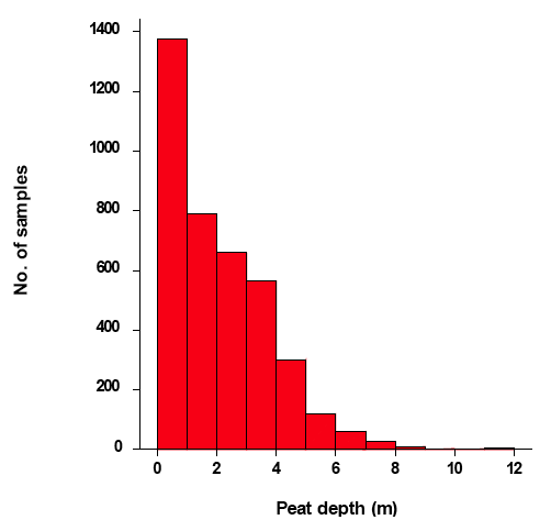
All depth data was recorded from a total of 77 'bogs' and the period of recording was from April 1969 until September 1979. Two bogs were omitted from the notes as one had only one depth record and the other was in England. Some of the 'bogs' were transects across large tracts of peatland rather than being a discrete bog. In the calculation of mean depths and variances, values recorded as zero were omitted as (i) these were not peat but mineral soil, (ii) these tended to be values recorded at the start of transects and hence marked the edge of the bog, and (iii) this was consistent with the protocol used in the ECOSSE project. About 17% of the remaining values recorded an organic layer less than 0.5 m and hence technically were not peat. However, these values were retained in the dataset as they represented variation in the depth at a spatial scale below which these variations could be mapped on the 1:250,000 map and as such contributed to the mean depth of the overall peat polygon. A summary of the raw data for these peat bogs is given in Appendix 1. Across the 3924 non-zero depthings, the mean depth was 2.19 m with a maximum depth of 12 m though this was exceptional (Figure 3.1.8). Excluding one peat bog (Din Moss), which exhibited a very large variance in depth (14.9 m ²), the mean variance was 1.76 m ², extending up to 6.1 m ² (Figure 3.1.9).

Figure 3.1.8 Histogram of peat depth distributions from survey data on 77 peat bogs

3.1.11. Power analysis

Using the data gathered in section 3.1.10, it is possible to perform a power analysis in order to estimate the number of samples required to obtain a value for a degree of precision in peat depth within those regions where data is missing. The results are summarised in Table 3.1.10. We have taken the mean depth of peat to be 2.28 m and the variance to be 1.93 m ², which are the mean values for the 77 peat bogs (Appendix 1). The table gives the number of extra depthings required to give a set precision and to obtain that value with either 95 or 99% confidence. For example, to be 95% confident of obtaining a mean peat depth that is within 5% of the true value will require nearly 600 individual values. This assumes that the variance in unknown areas is same as that in the known areas.

Figure 3.1.9 Histogram of variance (m ²) in peat depths for 76 peat bogs

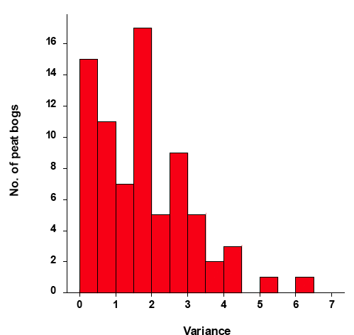
Table 3.1.10 Power analysis: number of samples required to obtain depth data with a given precision and with a specified confidence

Precision	Number of samples
	@95%	@99%
± 20 %	38	65
± 10 %	145	250
± 5 %	573	989

3.1.12. Conclusions

This study has used exploratory geostatistics to study the scales of variation in peat depths at five sites having three contrasting peatland types comprising:

• one basin peat
• one semi-confined valley side peat
• three sites with hill (blanket) peat.

The sampling designs on the sites used grid designs at 100 or 200 m with two of the hill peat sites sampled preferentially, along transects following proposed road construction routes. The basin peat has a range of spatial dependence between 400 and 650 m. The valley side peat studied apparently has no spatial dependence. Of the three hill peat sites, only site E has sufficient sample numbers for an estimate of a variogram model. This fact, combined with an inferred trend in peat depths on the other two peat sites leads to the conclusion that hill peats have a range of spatial dependence between 376 and 558 m. These variable results for fitting models indicate that there is not sufficient data for reliable modelling of the variogram.

We recommend that some effort should be made to identify the scales of variation in peat depths using sampling frames designed to capture different scales of spatial variation. The results suggest that a greater number of peatland examples should be examined over a wider geographical area to identify and separate regional components of spatial variation, which may be due to regional climatic differences, from local components of spatial variation, due to topographic or other short range factors which influence hydrology. Effort should be made to include study of the polygon boundaries between peaty and mineral soils, using for example, an indicator geostatistics approach with data on the presence and absence of a peaty layer.

A sensitivity analysis on the parameters needed to compute a total peatland C stock for Scotland showed decreasing uncertainty in the order dry bulk density > peat depth > peatland area > %C. Additional considerations were that both the available bulk density and %C values were not spatially explicit and that global values had to used based on limited data. Also, peat depth was partly reliant on measured values and partly on values estimated by expert judgement for areas of the country where depth values had not been determined. Accepting some assumptions about the country-wide applicability of values obtained from more restricted regions, the total C stock was estimated to be 1620 Mt with a 95% confidence interval of 1482-1757 Mt C.

A re-examination of archived data on peat depths revealed a wide range of variances across 77 peat bogs with a mean value of 1.93 m ². Using this value, a power analysis was used to compute the additional number of depth measurements required to compute a mean peat depth with a given precision and level of confidence. For example, to be 95% confident of obtaining a mean peat depth that is within 5% of the true value will require a minimum of 573 individual values. As indicated above the current uncertainty in total C stock is about ±138 Mt C (95% confidence). If we assume no strong regional trends in bulk density or %C, then such improvements in peat depth would reduce the uncertainty to about ±81 Mt C.

3.2. Peat depth simulations

3.2.1. Introduction

The mean peat depths of 341 peat bogs in Scotland were computed from data contained in soil survey memoirs, peat survey reports and Forestry Commission site surveys as outlined in the ECOSSE Report (Smith et al., 2007b). Expert judgement used this data, together with information on topography and any additional survey notes, to make an informed guess of the average peat depth for each polygon on the 1:250,000 scale soil map of Scotland (see also section 3.1.9). There are 20720 polygons on the digital version of the map; the subset of 1328 polygons estimated to have a mean peat depth greater than zero is reported on in this simulation study.

3.2.2. Summary of the polygon and peat bog data

There are two data sets

• Peat bogs: measured mean depths (cm) calculated from site peat survey measurements and reported on in the ECOSSE report. This set has the coordinates of the centroid of the data measurements and a mean depth for the peat. This set is referred to in this report as the data.depth.
• Deduced peat depths (cm) of map polygons. This set has the coordinates of the polygon centroid and the mean depth deduced by an expert. Referred to in the report as expert.depth.

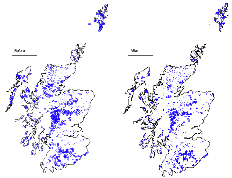
There is a difference in the geographical distribution of the two datasets (Figure 3.2.1). The data.depth map shows the location of peat polygons where we have actual measured depth data while the expert.depth map shows the location of those peat polygons for which we have no measured values and these have had to be derived from expert judgement. There are a large number of polygons in areas with few observed data for peat bogs, particularly in central Scotland and on the Inner and Outer Hebrides, i.e. the measured dataset tends to be rather patchy and not evenly distributed across the areas where peat occurs. The histograms of coordinates show different distributions in eastings and northings in more detail. The eastings plot shows that the measured data has been slightly biased towards the east while the northings plot indicates that there are data gaps around the centre of the country.

The mean depth of the peat bogs (data.depth) is 226 cm and the mean of the expert deduction for the peat polygons (expert.depth) is 169 cm (Table 3.2.1). A t-test, using the Welch approximation to degrees of freedom because of inequality in the variances, indicated that the difference in arithmetic means of 57 cm between these two sets is significant at the 95% confidence level. The same applies for the geometric means. The 95% confidence intervals in the arithmetic and geometric means are given in Table 3.2.2. These results indicate a significant difference in the global means (arithmetic and geometric) between the measured depths at peat bogs and the expert deduction for the polygons (Figures 3.2.2. and 3.2.3). The main reason for this is the mis-match in the spatial locations of the sampled peat bogs compared to that for the polygons (see on depth in section 3.1.9).

Table 3.2.1. Comparison of data.depth with expert.depth (cm)

	data.depth	expert.depth
Type of data	Mean depths in peat bogs	Deduced depths in peat polygons
Number	341	1328
Minimum	30	50
1 st quartile	120	75
Median	206	150
Mean	226	169
3 rd quartile	297	220
Maximum	843	702
Variance	16940	10080

Figure 3.2.1. Geographical spread of sites and summary histograms for data.depth and expert.depth

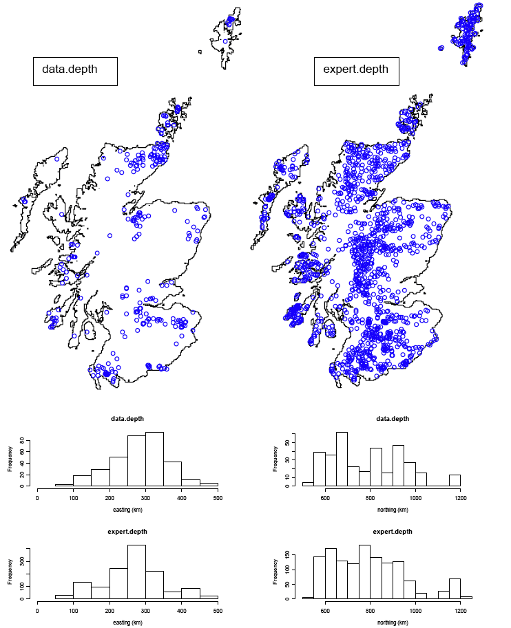
Table 3.2.2. Arithmetic and geometric mean depths (cm)

	data.depth	expert.depth
Arithmetic mean and 95% confidence interval	226.3 [212.4 - 240.1]	169.2 [163.7 - 174.6]
Geometric mean and 95% confidence interval	191.1 [179.2 - 203.8]	144.0 [139.7 - 148.5]

Figure 3.2.2. Histograms of data.depth and expert.depth (cm)

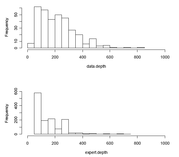
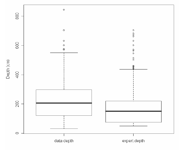
Figure 3.2.3. Boxplots of data.depth and expert.depth

3.2.3. Geostatistical study of peat depths in bogs and polygons

Variography of data.depth

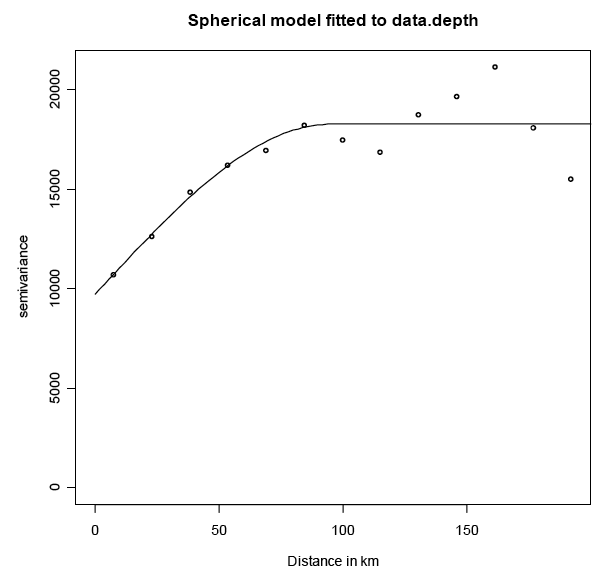
Variograms were computed for the mean peat bog depths (Figure 3.2.4) and indicate a range of spatial correlation around 100 km. A spherical model was fitted, having range parameter of 95.2km, nugget value of 9695 cm ² and sill of 8564 cm ².

Figure 3.2.4. Variogram model for data depth

Comparison of kriged estimate with expert deduction at polygon centroids

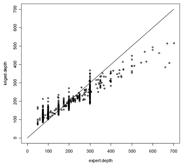
The variogram model and the peat depth data for the peat bogs were used to predict a value for depth at each of the 1328 polygon centroids using ordinary kriging. The expert depth values at the polygon centroids were removed before the kriging estimation. The statistics for the kriged predictions are compared to the expert deductions in Table 3.2.3. A t-test indicated no significant difference in the mean values at the 95% level. However, when kriged.depth is plotted against the original expert.depth (Figure 3.2.5), differences in the values at each end of the depth scale become apparent.

Table 3.2.3. Kriged prediction and expert deduction for peat depth (cm)

	Kriged.depth	Expert.depth
Type of data	Kriged depths in peat polygons	Deduced depths in peat polygons
Number	1328	1328
Minimum	73	50
1 st quartile	121	75
Median	158	150
Mean	172	169
3 rd quartile	204	220
Maximum	514	702
Variance	4230	10080

Figure 3.2.5. Kriged.depth plotted against expert.depth for polygon centroids

3.2.4. Bayesian geostatistical simulations

The model-based approach to geostatistics (Ribeiro and Diggle, 1998) was used in a simulation procedure to assess where the optimal sites for new samples would be. The measured peat depths (data.depth) were used to simulate 50 values at the polygon centroids. From these 50 simulations the mean depth and variance was calculated. The 24 polygons with the largest values for variance were selected. The simulated means were added to this set of 24 and a new simulation run performed using these additional 24 polygons as if they had been sampled. The procedure was repeated 3 times. Once 72 (3*24) bogs had been 'sampled' with simulated values, the variances were effectively reduced by around half (Figure 3.2.6). These results indicate that around 72 additional samples targeted at locations from the simulation effectively reduce the uncertainty in depth measurements by 50%.

3.2.5. Conclusions

The above study has demonstrated that using an analysis of the spatial statistics for peat depth it is possible to make a prediction of peat depth in areas where no measurements are available. Essentially, this relies upon distance to the nearest known values and clearly in areas where little data exists, the variance about the prediction increases. The expert judgement used in the original estimation of peat depths across the country similarly relies upon the depth in adjacent peat polygons where these are known. For this underlying reason, the agreement between the two approaches gives broadly similar results. However there was some consistent deviation, particularly at the deeper end where the expert system gave deeper peats. This is attributed to the expert system using additional information in its judgement, such as knowledge of the landscape and local topology and/or survey notes indicating 'deep' or 'shallow' peat. We conclude that the expert system gives a fair prediction for most peats and that the similarity in mean values indicates little difference in overall C stocks computed using either approach.

The simulation study has indicated that were 72 additional peat bogs sampled, targeted using the simulation results, the variances could be reduced by around 50%. This approach is also able to indicate the optimum location of these additional samplings, principally in the Western Isles and in central and north-west Scotland. While the current run considered increments of 24 additional bogs to give approximate locations, the optimum solution would be to use increments of one. However, the computational effort lies outwith the current project.

Figure 3.2.6. Variances of Bayesian simulations before and after first 24 samples added. Variances are proportional to the diameter of the plotted circles.

3.3. Report on targeted peat resampling

3.3.1. Introduction

This analysis is a general synopsis of the procedural and methodological considerations required when undertaking a survey of peat bogs, the logistical issues involved, the expected timescale and an estimate of costs when measuring the depth of peat and bulk density at 50 cm intervals, in a targeted sampling exercise.

3.3.2. Methodology

The standard and accepted methodology of measuring peat depths and sampling peat in order to characterise specific bogs involves two separate, but related stages - a) depthing on a grid pattern across the bog and b) sampling at 0.5 m vertical intervals, at between 5% and 10% of the observed depthing points.

Depthing

Following a reconnaissance survey of the area, a baseline is set out, usually along the longest axis of the bog. At fixed intervals along the axis, typically 100 m, the depth of peat is measured using interchangeable depthing rods of 1.5 m length which are inserted vertically into the peat until the underlying mineral or rock is encountered. Experience of staff in differentiating between mineral, rock and tree roots or wood fragments embedded in the peat is essential. The depth of peat is then recorded and the location of each point is also recorded using a Global Positioning System ( GPS). Wooden pegs can be inserted at these points for relocation purposes when undertaking sampling. Extending from the baseline, depth and location measurements are made on a uniform grid across the bog. Variation of peat depth throughout the year because of differing hydrologic conditions is known to occur, but due to the relative accuracy and detection limits of the depthing rod technique and the measurements made, which relate specifically to the conditions on the day, little can be done to accommodate or assess this phenomenon, using the methodology discussed.

Sampling

At the selected depthing points, which are usually sited to give an even coverage of the area and to provide an agreed minimum sampling density, peat samples are taken using a Russian sampler at 0.5m intervals from the surface to the bottom of the peat deposit. This is a chamber of known volume which is attached to interchangeable rods and is inserted to specific depths within the peat profile from which a sample of peat is extruded. After removal of the chamber the peat is examined for degree of humification/decomposition (von Post classification) and samples are carefully extracted, bagged and labelled with site, location and depth range for bulk density and chemical analyses.

Additional characterisation

There could be added value to the resampling program to include additional characterization of the peatland at each sampling point. Such parameters might include a full peat profile description, a more detailed vegetation/plant species survey, assessment of peat erosion, assessment of local negative impacts such as grazing, peat cutting, fire incidence, as well as any additional chemical characterisation of the peat samples uplifted. Such further characterisation would incur additional costs, which are not included here.

3.3.3. Logistics

The logistics of undertaking such an exercise are considerable and are briefly outlined.

• The bogs/polygons to be sampled have to be identified.
• Construct agreed protocols and methodologies which meet the objectives of the project.
• List required of experienced personnel and equipment.
• Acquire/purchase relevant equipment.
• The ownership of the land relevant to the bog/polygon has to be acquired. This is not always readily available, may involve more than one owner and is often time consuming.
• Contact the owner by letter, explaining the reason for the work, how the work is to be undertaken, how long it will take and when the work is proposed to be carried out. Provide various options for replies e.g. stamped self-addressed envelope, telephone or email.
• Draw up provisional timetable of fieldwork taking into account available personnel, distribution and size of bogs/polygons.
• On receipt of replies granting access, finalise timetable of fieldwork, minimising travel and costs, and make arrangements for receipt and analyses of samples.
• Undertake fieldwork

(i) Depth recording

(ii) Sampling for bulk density, C/N analyses and humification assessments.

• Analyses of samples
• Data input into database
• Analyses of results
• Report and presentation of results.

3.3.4. Logistical Issues

Many issues arise when planning and undertaking such work, some of which can be foreseen and appropriate provision made, others are not e.g. inclement weather, unsafe ground conditions, breakage of equipment, rods becoming separated at depth. Some of the practical issues which would have to be taken into account when planning are:

• The scale of the 1:250,000 scale soil map which forms the basis of this work, does not allow a suitably accurate enough picture of the actual size of the bog when assessing timings and costings.
• Work is strenuous and requires at least two people for all field aspects of the work.
• Obtaining information on ownership of land and gaining access can be time consuming and problematic.
• The location and management of the bog may impose restrictions of access (nesting birds, shooting seasons and lambing) to times of the year, unsuitable for sampling.
• Accessibility of the bog from roads and the nature of the terrain can be difficult, curtailing the volume of work which can be undertaken. Previous peat surveys involved more staff and a tracked vehicle which is no longer available to traverse the bog.
• The depthing and sampling rods are difficult to manually carry over long distances and across steeply sloping land. For deep bogs more than two people may be required.
• Manufacture or acquisition of additional Russian samplers would be required if more than two teams were used (only two are extant which makes no allowance for loss or breakage).
• Variability across the bog in depth and nature of peat.
• Where root and wood fragments are present within the peat, several attempts may be necessary to ascertain the depth of peat to the underlying mineral substrate.

3.3.5. Timescales

This is dependent upon many factors - the size and number of bogs to be surveyed (Objective 1), the location, the grid size, distance to bog, the terrain and the depth of peat.

However it is estimated that once on site where depths do not exceed 3 m, a maximum of 22- depth recordings could be undertaken in one 8.5 hour day, allowing time for assembling rods, measuring the depth, recording location, dissembling rods and walking to the next recording point. Where depths exceed 3 m, a maximum of 17 points would be a realistic figure.

This assumes 9.5 hours daylight, weather is dry, there are no obstacles such as ditches to traversing the site and there is no walk in time from the vehicle.

Sampling is more time consuming than the depthing stage because of:

• heavier and more cumbersome equipment that has to be assembled and dissembled at each sampling site
• the process of sampling, bagging and labelling,
• undertaking and recording humification/decomposition assessments
• distance between sampling sites will be greater

It is estimated therefore, that a maximum of 6 sampling points across a bog could be visited in one day. This would be reduced if the depths encountered typically exceed 3-4 m.

Depending on location and distance from Aberdeen, travelling to and from many of the bogs will entail a minimum of 1 day but often two days. In a normal working week this equates with a maximum of 68-88 depth recordings (bog area of 68-88 ha if a 100 m grid is adopted) or 24 sample sites.

Taking into account the issues mentioned previously, 34-44 points and sampling 12 points on one bog per week would seem to be a realistic expectation. Reducing the depthing points to 17-22 and the sampling points to 3, could enable two bogs to be covered per week, provided that the travelling distance between the two was minimal.

3.3.6. Deliverables

Adopting the methodology described would allow the following deliverables:

• A map detailing depths across the bog on a grid basis with sampling sites located.
• Tables of location, sample depth, humification/decomposition assessments, bulk density and %C and N at each of the sampling sites.
• Estimate of C stocks for the bog.
• Report of work and results.

3.3.7. Costs

The costs are dependent upon many of the issues raised previously, but particularly the distance from Aberdeen, the size of bog, depth of peat and the number of samples. Outsourcing of work might reduce travel costs, but the need for training and equipment to ensure consistent results would offset any benefit of subcontracting.

However, assuming a week's fieldwork (depthing 44 points and sampling 12 points) for two staff (Band E @ £479 per day and Band C @ £392 per day), with associated travel and subsistence, analyses of 72 samples (peat 3 m depth, 6 samples per point) for loss on ignition and total C and nitrogen with the necessary drying, sieving and milling, plus office time for preparatory and data manipulation work, an estimated minimum cost associated with one week's fieldwork is approximately £8700. The number of weeks' fieldwork and total costs are based upon the outcomes of Sections 3.1 and 3.2 whilst the need for additional staff, more samples, ferry trips and the purchase or manufacture of equipment will increase costs accordingly.

A provisional estimate is that an additional 72 spatial locations would reduce the variance on the depth estimates by 50% (see Section 3.2.5). At the same time, power analysis indicates that a total of ca. 600 depth values should give an acceptably precise mean depth (see Section 3.1.12). Hence the indication is that it is better to have fewer depth samplings, say 8-10, at a greater number of locations (peat polygons). However, the results of the spatial analysis (Section 3.1.8) would suggest that sample points should be at least 500 m apart rather than the traditional 100 m to avoid spatial autocorrelation. (To some extent this might need to be adjusted to take into account practicalities and the size of the particular peat area.) As result there would be an offset between fewer sampling points and more walking between points. Hence total costs, assuming 36 weeks of field work would be of the order of £313k.

3.3.8. Conclusions

To undertake a comprehensive targeted peat sampling programme will be time consuming and costly in terms of salaries, equipment acquisition and analytical costs. The costs and timescale involved should be considered against the benefits ensuing from collecting such data. The data collected during the current NSIS_2 resampling programme will provide some information on the thickness and depth of horizons, which combined with bulk density analysis and %C values, will allow C stocks for the soil profiles sampled to be calculated, enhancing the national soil datasets and the associated variability studies will also give an insight into the range of values around a point. The NSIS_2 work will also provide information on the thickness of organic horizons within organo-mineral soils and using hand held augers, the thickness of peat deposits at each site can be assessed to 2m depth, again enhancing previous information and C stocks. However to transport actual peat depthing rods to each site in conjunction with the required NSIS_2 equipment, is not thought a feasible proposition within current budgets and any additional sampling of peat below 1 metre should be undertaken as a separate exercise as outline above. Such an exercise would allow the known uneven distribution of data, both across the country (east to west) and between peat types (basin and blanket) to be built into the sampling programme, and would reduce the uncertainty in C stock measurements by at least 50% (equivalent to ca. 50 MtC), as well as providing some validation (or otherwise) for some of the assumptions used in the current C stock estimates about more locally-obtained parameters being applicable across the country. Using the data from geo-statistical analyses (Section 3.1), the necessary work is estimated to cost of the order of £313k.

3.4. Evaluation of use of archived dry bulk density values for peat bogs to determine C stocks values retrospectively

3.4.1. Introduction

There exists in the archived records of the surveys of the Scottish Peat Committee some data on what is termed "bulk density" but what is actually a laboratory bulk density, or particle packing density, of dried and milled peat, together with recorded peat moisture contents, ash content and humification indices on the von Post scale. Here we investigate the possibility of using this data to reconstruct the actual field dry bulk density using pedotransfer functions. The benefit of this approach is that the archived data extends to the base of many peat deposits and so could give data on bulk density at depths greater than 100 cm, as well as giving an indication of how bulk density may vary (or not) with depth in different peatland forms. This exercise includes some limited sampling of different peat sites in order to verify the relationships between the laboratory bulk densities and field bulk densities. We also utilise data from the first phase of the NSIS_2 resampling, where there is sufficient sample volume available for this project.

3.4.2. Methodology

The initial step in this exercise was to translate the archived data into computer format. The data exists as figures within the reports (Volumes I to IV) of the Scottish Peat Committee (Department of Agriculture and Fisheries for Scotland, 1964; 1965a; 1965b; 1968). While scanning the data or using a digitizing tablet was considered, the most efficient way was to measure the length of the bars on the figures with a ruler, measure the scale and enter the figures into an Excel spreadsheet. From this the actual values could be computed. The data entered were the "bulk density" (henceforth referred to as "laboratory bulk density"), moisture content, ash content and humification index on the von Post scale. Values were recorded typically every 50 cm down the peat profile to the bottom of the peat layer (for the deepest this was 9.5 m) and the dataset contained over 80 profiles.

The second step was to derive a pedotransfer function whereby the archived data could be used to give values of dry bulk density down the peat profiles. Laboratory bulk density is not normally measured in contemporary analysis; its value related more to peat extraction for fuel use and so was of relevance to the post-war Scottish Peat surveys but not so any longer. The precise protocol for its measurement is unfortunately no longer available. Even interviewing a number of contacts with considerable history in peat survey (R.A. Robertson, P.D. Hulme and J. Anderson) did not bring to memory its exact nature except that the dried and milled peat was compacted by shaking it on a ratchet-like device on a wheel that was turned. Comparison with the literature (Päivänen, 1969) revealed that there were several variants on the methodology. It was decided to adopt the following protocol:

1) The peat was air-dried at 27ûC and subsequently at 105ûC.

2) The dried sample was hammer-milled using a 1 mm grid on the mill.

3) A sample of 20-30 ml was placed into an adapted 50 ml syringe body and tapped 30 times by hand on the bench from a height of 3 cm (A preliminary test indicated that this consolidated the sample to a constant volume).

4) Both the volume and weight of the sample was recorded and from these the laboratory bulk density could be calculated.

The laboratory bulk density was determined for a number of peat samples for which (field) dry bulk density had also been determined:

1) Samples (28) from two basin peats (Middlemuir and Red Moss, Netherly) collected using a Russian sampler to a maximum depth of 5 m. The humification index and moisture content was also recorded.

2) Samples (20) from eleven NSIS_2 sites which were peat. These were necessarily only to a maximum depth of 1 m. Humification index and moisture content were not available.

A further set of data from Shetland, Allt Mharcaidh and Glensaugh (supplied by Zoë Frogbrook) were added where both bulk density and moisture content values were known. The original samples were not available for laboratory bulk density determination.

Linear regression and multiple linear regression between the various parameters were performed using Genstat 8.

3.4.3. Results

The results of regression analysis revealed a significant but not particularly strong relationship between dry bulk density and laboratory bulk density (Figure 3.4.1). The relationship could be improved by removing one or two data points which had come from near surface samples and which had particularly high dry bulk density values, e.g. the value over 0.2 came from a sample that represented an old cut-over surface that had previously been dried and consolidated. However, the regression was still not very good (data not shown).

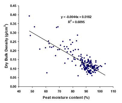
During the process of regression analysis, it was found that that the relationship between dry bulk density and moisture content was much closer (Figure 3.4.2). The figure gives the regression for the values obtained from the two basin peats; a quadratic (polynomial) fit was slightly better than a simple linear regression and an r-squared in excess of 0.99 was obtained. A second larger dataset from blanket peat (Shetland, Allt Mharcaidh and Glensaugh) gave different regression line having greater scatter and with an r-squared of 0.61 (data not shown). It was decided to combine the two datasets to give a general regression that could be applied to the archived moisture content values (Figure 3.4.3). The combined dataset also had an r-squared of 0.61 and only a linear fit was justified. Some samples showed lower moisture contents than might be expected. Closer inspection indicated that these samples had lower wet bulk density values also and hence were from unsaturated horizons that contained an appreciable air-space.

Further regression analysis was performed to ascertain if the relationships between dry bulk density and peat moisture content could be improved further by the addition of the humification index or of laboratory bulk density (in a multiple linear regression analysis). The results indicated that the addition of the laboratory bulk density gave some improvement but not the addition of the humification index. However, the number of samples where these additional parameters were known was limited and hence it was preferred to use the larger dataset of moisture content alone as the predictor of dry bulk density.

Figure 3.4.1 Regression of dry bulk density on laboratory bulk density for a set of peat samples

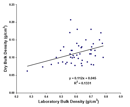
Figure 3.4.2 Regression between dry bulk density and moisture content using data from two basin peats.

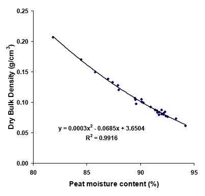
Figure 3.4.3 Regression between dry bulk density and moisture content using data from both basin and blanket peats.

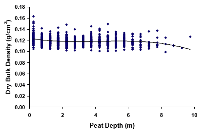
The final step was to apply the regression relationship obtained from Figure 3.4.3 to the archived data on peat moisture content in order to calculate a dry bulk density. This would enable characterization of how this parameter may vary with depth. Figure 3.4.4 shows the variation in bulk density with depth using 918 datapoints from 86 peat profiles taken from a total of 32 peat bogs. There is an underlying assumption that the pedotransfer function that was obtained using data from shallower peat profiles can be applied to the deeper peat profiles of the archived dataset; the regression dataset had a mean depth of only 48.7 cm (range 7.5-485 cm) while the archived data goes down to nearly 10 m. However, if this is accepted then the data shows little variation of bulk density with depth. There is slight evidence of a minimal decrease with depth; the fitted line is a cubic polynomial which is a significantly better fit than a linear regression. The suggestion is a slight increase in bulk density at the surface and a slight decrease below 8 m though the data points here are few. Taking means over the depth ranges as used for the C stock calculations gives estimated bulk density values (g cm ^-3) of 0.125 (0-30 cm), 0.118 (30-100 cm) and 0.118 (100+ cm). These are very close to the mean bulk density values actually used in the C stock calculations from a more limited set of measured bulk density data, 0.134, 0.120 and 0.109, respectively, and give some confidence to the application of these values.

Figure 3.4.4 Predicted dry bulk density, using the regression against moisture content, and its variation with peat depth.

3.4.4. Conclusions

A pedotransfer function may be derived that enables dry bulk density to be estimated from peat moisture content. A restriction is that the peat samples should be from the saturated zone or at least have a wet bulk density in excess of 0.85. Since we are here interested in bulk density changes at depth, this restriction does not interfere too much with its application. The application of this function to a set of archived peat moisture content data yields bulk density data that is comparable to that actually used in the national C stock calculations and gives some credibility to these bulk density values. Additionally, it suggests that bulk density does not vary markedly with depth in these peat deposits so that surface values may be used with more confidence for deeper deposits where measured values are largely absent.

3.5. Costs and benefits of GPR and Lidar to measure peat depth and the potential for using these methods to monitor changes in soil carbon stocks in the peatlands of Scotland

3.5.1. Introductio

The collection of data related to the measurement of peat depth and monitoring of peat stocks has been traditionally carried out by intensive and expensive field work. Whilst field work will remain an important component of any future work in this area, not least for validation purposes, new remote techniques may enable more measurements to be undertaken at less cost. This short analysis reviews the use and potential of the Ground Penetrating Radar ( GPR) and LIDAR ( Light Detection and Ranging) technologies both for measuring peat depth and to monitor changes in peat depth in Scotland. The Scottish Government is currently funding two pilot projects to evaluate the feasibility of using satellite derived information to measure the extent of erosion and greenhouse gas emissions from Scottish peatlands. This work is due to complete in 2009 and will help to inform the Scottish Government on the value of this new technology in supplementing more traditional and costly field measurements.

3.5.2. Ground Penetrating Radar ( GPR)

Ground Penetrating Radar (or GPR for short) is the general term applied to techniques which employ radio waves, typically in the 1 to 1000 MHz frequency range, to map structure and features buried in the ground. It is often used in the building industry to determine and inspect the general arrangement of construction, changes in material type, location of structural steelwork and layer thickness.

It is a high resolution, field-portable geophysical method that produces graphic sections of subsurface structure. Typical site investigation applications include accurate location of voids and buried obstructions; mapping subsurface soil and rock interfaces and defining buried archaeological structures. The method can also identify ancient landfill sites and detect buried hazardous waste. In man made built environments, use of GPR is quite straightforward and machine use and data capture can be at rates not much slower than normal walking pace, but ease of access could be a significant constraint in peatland environments. This will be discussed more fully later.

Applications in Soils Research

The performance of ground-penetrating radar ( GPR) in soils strongly depends on soil electrical conductivity (Doolittle et al., 2007). Electrical conductivity is the ability of a material to transmit (conduct) an electrical current and is expressed in the units milliSiemens per meter (mS/m). Soil electrical conductivity measurements may also be reported in units of dS/m which is equal to the reading in mS/m divided by 100. Soils having high electrical conductivity rapidly attenuate radar energy, which restricts penetration depths and severely limits the effectiveness of GPR. GPR can offer a number of advantages over traditional methods of digging soil pits as these are destructive, time consuming and only provide single point sources of information (Knight 2001, Holden et al., 2002). For specific applications such as measuring and mapping soil water content, GPR is a technique that is intermediate in resolution between the detailed scale of time domain reflectometry ( TDR) and the small scales that remote sensing using air photographs or satellites can handle (Huisman et al., 2002).

A number of soil properties are known to affect electrical conductivity in soils (Geonics Limited 1980). These include:

• Pore Continuity - Soils with water-filled pore spaces that are connected directly with neighbouring soil pores tend to conduct electricity more readily. Soils with high clay content have numerous, small water-filled pores that are quite continuous and usually conduct electricity better than sandier soils. Compaction normally increases soil electrical conductivity, presumably by reducing air space within the soil matrix.
• Water content - Dry soils are much lower in conductivity than moist soils.
• Salinity level - An increasing concentration of electrolytes (salts) in soil water will dramatically increase soil electrical conductivity. The salinity level in most humid regions such as the Corn Belt is normally very low. However there are areas that are affected by Ca, Mg or other salts that will have elevated electrical conductivity.
• Cation exchange capacity ( CEC) - Mineral soils containing high levels of organic matter (humus) and/or 2:1 clay minerals such as montmorillonite, illite or vermiculite have a much higher ability to retain positively charged ions (such as Ca, Mg, K, Na, NH4, or H) than soils lacking these constituents. The presence of these ions in the moisture-filled soil pores will enhance soil EC in the same way that salinity does.
• Depth - The signal strength of EC measurements decreases with soil depth. Therefore, subsurface features will not be expressed as intensely by EC mapping as the same feature if it were located nearer to the soil surface.
• Temperature - As temperature decreases toward the freezing point of water, soil EC decreases slightly. Below freezing, soil pores become increasingly insulated from each other and overall soil EC declines rapidly.

Ground penetrating radar ( GPR) has been used as a pedological tool in the United States since 1978 (Doolittle and Collins 1995). Principal uses have been to estimate the variability and taxonomic composition of soils, chart the lateral extent, and estimate the depth and thickness of soil horizons and geologic layers and to map and interpret soils. All soils are not equally suited to GPR techniques. A Ground-Penetrating Radar Soil Suitability Map has been produced for the United States based on taxonomic criteria, clay content, salinity, sodium absorption ratio, and calcium Cate content (Doolittle et al., 2007). The map is based on over twenty-five years of field observations made throughout the United States and soil attribute data contained in the State Soil Geographic ( STATSGO) database. The map limits areas that are rated as being "Unsuited" for GPR to saline and sodic soils, reassesses calcareous and gypsiferous soils, and provides a mineralogy override for soils with low activity clays. This map can be used to assess the relative appropriateness of GPR for soil investigations within comparatively large areas of the conterminous United States. No similar analysis has been undertaken nor map produced for the UK.

Many of the specific GPR applications have been in relation to soil water content in mineral soils (rather than peat soils, which is the focus of this report). Weihermueller et al. (2007) used two ground penetrating radar ( GPR) techniques to estimate the shallow soil water content at the field scale. The first technique is based on the ground wave velocity measured with a bistatic impulse radar connected to 450 MHz ground-coupled antennas. The second technique is based on inverse modelling of an off-ground monostatic TEM horn antenna in the 0.8-1.6 GHz frequency range. The aim of the study was to test the applicability of the ground wave method and the off-ground inverse modelling approach at the field scale for a soil with a silt loam texture. Both methods produced disappointing results and did not provide adequate spatial information on soil water content variation at the field scale. The main reason for the deviating results of the ground wave method was the poor data quality due to high silt and clay content at the test site. Additional reasons were shallow reflections and the dry upper soil layer that cannot be detected by the ground wave method. In the case of off-ground GPR, the high sensitivity to the dry surface layer is the most likely reason for the observed deviations. The off-ground GPR results might be improved by using a different antenna that allows data acquisition in a lower frequency range.

Strobbia and Cassiani (2007) used GPR as a tool to quickly obtain soil moisture content over large areas. The technique was applied to a mountain slope with a 1-m soil cover where repeated measurements over time, inverted by conceptualizing the soil as a single guiding layer, lead to estimates of the GPR wave velocity and thickness varying over time. They developed a multilayer GPR waveguide model and although this did partly overcome the model error arising from using a single-layer forward model - it underestimates the total soil thickness because the inversion is sensitive mainly to the layer with the lowest velocity (the wettest layer) - it did not fully overcome it. They then used a multilayer forward model to invert the actual field data. There was still some uncertainty about the position of such a layer in the layer sequence.

Other studies in the area of soil water content include that of Lunt et al. (2005) who concluded that GPR has the potential for monitoring soil water content over large areas and under variable hydrological conditions. This was done by comparing volumetric water contents from calibrated neutron probe logs with estimates produced from GPR reflections. Although they do not state it explicitly, they do not seem to advocate the technique as a substitute for field studies but rather to complement and provide a focus for them. GPR can provide continuous high-resolution data that chart depth to water tables in coarse textured soils (Doolittle et al., 2006).

GPR has also proved useful in soil pollution monitoring and in contributing towards describing the spatial distribution of pollutants in an industrial area in Southern Italy (Chianese et al., 2006). In a study investigating its potential use in identifying soil compaction, Petersen et al., (2005) demonstrated that loamy soils that have a higher risk of compaction could be differentiated by GPR from those with a lower risk, for example, sandy soils. However, they did not demonstrate whether compacted soils could be identified as the deeper soil horizons (below 30 cms) in the study area showed only uniformly strong compaction with little contrasts.

Applications in peat soils

Applications of GPR in peat soils have been carried out largely by Finnish and Canadian researchers in the measurement of peat depth and measurement of gas accumulation and release in peats, whilst work on the location and analysis of the connectivity of underground pipes in peat has largely been carried out in England.

Comas et al., (2007) reported that that GPR is a useful tool for assessing the spatial distribution, temporal variation, and volume of biogenic gas deposits in peatlands. They found that (1) changes in the two-way travel time from the surface to prominent reflectors allow estimation of average gas contents and evolution of free-phase gas ( FPG); ( 2) peat surface deformation and gas flux measurements are strongly consistent with GPR estimated changes in FPG content over time; ( 3) rapid decreases in atmospheric pressure are associated with increased gas flux; and ( 4) single ebullition events can induce releases of methane much larger ( up to 192 g m ^-2) than fluxes reported by others. The same authors subsequently found that GPR in combination with other techniques provided insights into the spatial and seasonal variability in production and emission of biogenic gases from northern peatlands (Comas et al., 2008).

Natural underground soil pipes are common in peat and can play a significant role in catchment drainage where peat forms a significant component. Holden et al. (2002) compared data on pipes identified by GPR and verified by manual measurement and found that that pipes can be located in the soil profile with a depth accuracy of 20 to 30 cm. Generally pipes smaller than 10 cm in diameter could not be identified using the technique although modifications could allow enhanced resolution. GPR demonstrated that pipe network densities were much greater than could be detected from surface observation alone. Thus, GPR provides a non-destructive fast technique which can produce continuous profiles of peat depth and indicate pipe locations across survey transects. Subsequent work (Holden 2004) has demonstrated that GPR in combination with a tracer solution can identify connectivity within the pipe network and travel times within that network.

Most GPR applications on peat have been to test how well the technique can identify different layers within it, in other words its stratigraphy, and whether it can measure the total depth of peat to the underlying mineral material. Research by Comas et al. (2005) suggest that GPR and terrain conductivity measurements reveal a close correlation between the location of water-filled pools and stratigraphic/lithologic features in Caribou Bog, a 2200-hectare peatland in central Maine. The geophysical profiles, supported by coring, define the general peatland stratigraphy as till underlain by glacio-marine sediment overlain by organic-rich lake sediment transitioning into terrestrial peat. Similarly Slater and Reeve (2002) working on the same bog integrated GPR with direct measurements of peat stratigraphy from probing, fluid chemistry, and vegetation patterns in the peatland. They concluded that GPR was an excellent method for delineating peatland stratigraphy and prominent reflectors from the peat-lake sediment and lake sediment-mineral soil contacts were precisely recorded up to 8 m deep. Comparison of the bulk conductivity images with peatland vegetation revealed a correlation between confining layer thickness and dominant vegetation type, suggesting that stratigraphy exerts a control on hydrogeology and vegetation distribution within this peatland. Their understanding of the hydrogeology, stratigraphy, and controls on vegetation growth in this peatland was much enhanced from the geophysical study.

Thiemer and Nobes (1994) carried out geophysical surveys and chemical analyses on cores in three Ontario peatlands. They found that the dielectric permittivity in peats is largely controlled by the bulk water content and that GPR can detect changes in water content greater than 3%, occurring within a depth interval less than 15 cm. The principal peatland interfaces detected by GPR are the near-surface aerobic to anaerobic transition and the peat to mineral basement contact. The potential for the successful detection of the basement contact using the radar can be predicted using the radar instrument specifications, estimates of the peatland depth, and either the bulk peat or the peat pore water electrical conductivities. Predicted depths of penetration of up to 10 m exceed the observed depths of 1 to 2 m so the full capability of the technique was not fully tested in this study. At the third one, on the other hand, it was observed that, as predicted, a 100 MHz signal will penetrate to the base of a 2 m thick peat but a 200 MHz signal will not.

Jol and Smith (1995) used GPR in site assessment for the placement of pipelines crossing peatland. This built on previous work that demonstrated the use of GPR in the assessment of the thickness and volume of peat as a fuel resource and horticultural material in Scandinavia and Canada. Several GPR surveys assessed the thickness of the peat along two oil pipeline right-of-ways. Results show the peat-sand contact as irregular and undulating, ranging from 0 to 3.7 m deep. Each survey, 460 and 550 m long, was completed in two hours. Such results from 1 m station spacings (sampling interval) can considerably reduce the uncertainties in planning and placement of oil, gas, and water pipelines crossing peatlands. Significantly the authors argue that the results indicate that thickness variations of peat can be detected more effectively in terms of quality of results, lower cost, and less time with GPR than with a peat probe or by coring.

Hanninen (1992) wrote a major review of the applicability of ground penetrating radar (and radio wave moisture probe techniques) in practical research work between 1983 and 1990. The primary aim was to examine the practicability of ground penetrating radar antennae. Their main findings were that

• Ground penetrating radar provides continuous cross-sectional data on the depth of a mire, a good picture of the quality of its bottom and indications of the underlying mineral soil type. Together with location data, such a cross-section allows extremely accurate depth maps to be constructed for the site concerned.
• The method also constitutes a rapid means of examining open, unditched peatland areas, but is slower to use in forested mires with a dense network of ditches.
• Of the antennae available at that time, those of frequency 80, 100, 120 and 500 MHz lend themselves best to peatland investigations. The first three types are best suited for measuring peat layer thickness in extensive unditched peatland areas, while a 500 MHz antenna provides accurate data on the mire surface and moisture fluctuations inside the peat. The results can be improved markedly by digital processing of the radar cross-section, especially if a 500 MHz antenna has been employed.
• Possibly most significantly, the authors claim that the depth data obtained using ground penetrating radar are markedly more accurate and detailed than those obtained by traditional means.

Wastiaux et al. (2000) and Doolittle et al. (1990) have also undertaken peat bog surveys using GPR. Wastiaux et al., working on a 800 ha area of drained peatlands in the Hautes-Fagnes (Belgium), found that GRP 'provided very accurate information about the subsurface relief and the thickness and extent of the peat deposit, as well as stratigraphical information and suggestions of possible links between subsurface, hydrology and present vegetation'. Doolittle et al. used GPR to estimate peat thickness and peat volume within a kettle bog in Plymouth County, Massachusetts, USA.

3.5.3. Light Detection and Ranging technology ( LIDAR)

LIDAR is a remote sensing technique that uses laser light in much the same way that sonar uses sound, or radar uses radio waves . The journey time of the laser beam, from leaving the instrument to its return after reflection, is measured and - knowing the speed of light - a distance can be computed between the aircraft and the ground . It produces very high resolution surfaces and has been used in a number of ecological applications for example in forestry for measuring tree height and in flood risk studies. Applications in the study of soils and particularly in peat are very scarce but those that have been sourced are referenced here. Two good sources of information on the technical and applied aspects of LIDAR can be found at

http://www.forestry.gov.uk/forestry/INFD-6RVC9J and

http://www.snh.org.uk/pdfs/publications/commissioned_reports/F02LG15.pdf

In terms of quantifying peat resources, LIDAR [or as it is sometimes termed Airborne Laser Scanner ( ALS)] produces a very detailed and accurate representation of the ground surface. However this information has to be used alongside peat depth data collected by traditional ( e.g. coring or drilling) or remote methods such as GPR in order to generate a 3 dimensional representation of bogs. From this, total volume of peat can be estimated and when combined with data on soil C content and bulk density, C stocks can be derived.

A case study from Ireland (Lenihan 2008) used three steps:

1. process LIDAR data in GIS software to create a top surface for a particular bog. The data are accurate to 0.075m.

2. peat depth measurements collected in 1950 were entered into the GIS software to create a bottom surface.

3. using modelling functions in ESRI Arc GIS 9.2, subtract the one from the other to create a predicted peat depth map.

A similar study has already taken place in Indonesia within a tropical peatland (Boehm and Frank 2008). The ALS data were accurate to +/- 15 cm in elevation and to 0.5 m in the x and y directions and, the authors argue that 3-5% of the laser beams penetrate the peat swamp forest. This allowed them to produce a true topographic surface of the peat. Each flight track was GPS recorded. Peat depth readings were taken on a 500 x 200 m grid and GPS reading recorded at each point on the grid. In another part of the peatland, cores were taken every 700 m though access through the peat swamp forest was very difficult. Two georeferenced datasets were thus obtained albeit with radically differing levels of resolution and accuracy. Considerable computing power and expertise are required to analyse these data and to produce the 3 dimensional representation of the bog. Although the extent of the bog is not stated explicitly, from data presented it is of the order of 40 km long. Given the difficulties of access on this site, the obtaining of ALS data probably was the difference between the project being feasible at all.

An on-going project in the Peak District National Park in England is investigating the use of LIDAR along with other remotely sensed data to predict catchment sediment flux (Evans and McMorrow, pers. comm.). The overall aim is to assess the usefulness of pattern analysis of remotely sensed data to assess connectivity between peat gullies and their role in sediment flux. Clearly the capability of LIDAR data to produce accurate DEMs and therefore the degree of connectivity between gullies is fundamental to the success of this initiative.

LIDAR has also been used by Haycock et al. (2004) to classify the morphology and dynamics of the peat surface within a National Trust estate and then apply new topographically derived flow and network propagation models to map the drainage network of the landscape. From this information and the ability to classify the depth and drainage information of the gullies they were able to identify the critical gullies within the estate, select appropriate gully blocking techniques and then develop operational working plans that assist in the air-drop of materials to key locations.

3.5.4. Other methods

Although this report was asked to focus on the potential of GPR and LIDAR in peatland survey and monitoring, some other techniques emerged during the literature search and perhaps should be considered as part of the portfolio of techniques available. It should be recognised that most of the examples cited below have not been tested in peatland but are reported here as potential non-destructive techniques.

Radio wave moisture probes

Radio wave moisture probes have been used with the aim of examining their application in the measurement of peat moisture, bulk density and energy content in hydrologically different mires (Hanninen et al., 1992). The practicability of the radio wave moisture probe was examined by comparing the probing results with those obtained using a volumetric piston sampler and analysed under laboratory conditions. Following the collection of 4434 probe measurements and 739 volumetric samples taken from mires in 13 local government districts they were analysed for peat type, humification, moisture content, bulk density, ash content, heating value, and in some cases sulphur content. A radio wave moisture probe was used to measure attenuation, frequency and quality factor (Q value) in peat, of which the first can be used to calculate moisture content, bulk density and energy content. It was concluded that the method allows more accurate measurement of energy content and bulk density in peatland areas, as the number of measurements required in the latter case can be increased essentially without any rise in research costs. For example a group of 2-3 persons can perform 3-4 times more bulk density measurements in a day than by the traditional method, and the number of volumetric samples needed can be reduced by 30-50%. Cross-sections describing the moisture, solid matter and energy content in peat can be created and mire-specific maps printed on the basis of the results obtained.

Electromagnetic induction ( EMI)

Electromagnetic induction has been compared and contrasted with GPR with respect to its capability in rapid, extensive and non-destructive mapping of diagnostic subsurface features and soil series map unit boundaries (Stroh et al., 2002). In contrast to GPR, EMI consistently distinguished boundaries of soil map units. In several instances, gradients or contrasting inclusions within map units were also identified. In addition, the location and boundary of calcic or cambic-horizon inclusions embedded within a laterally co-extensive and well-developed argillic horizon were consistently predicted. However, correlations between EMI assessments of apparent conductivity ( ECa) and soil properties such as CEC, pH, particle size distribution and extractable bases were low ( i.e., explained <6% of the variance), or non-significant. As a result, EMI has a high prospecting utility, but cannot necessarily be used to explain the basis for edaphic contrasts. Results suggest EMI can be a cost-effective tool for soil survey and exploration applications in plant ecology. As such, it is potentially useful for rapidly locating and mapping subsurface discontinuities, thereby reducing the number of ground truth soil samples needed for accurate mapping of soil map unit boundaries. There is no evidence that the technique has been used on peatland soils.

Time domain reflectometry

In a similar fashion, GPR was compared with time domain reflectometry ( TDR) by Huisman et al. (2002). They demonstrated that GPR can measure soil water content variation as expressed in a variogram produced by the heterogeneous irrigation of ground using sprinklers of various intensities. Additionally they have demonstrated GPR is better that TDR for mapping features > 5 m in soil water content. GPR has also been utilised to investigate its utility in identifying depth to a ground water table. Roth et al. (2004) demonstrated that discontinuities in soil could be identified and a local water table located, all verified by soil coring and water table measurement in the field. They advocate its use as a initial screening tool to help find optimal locations for field based measurements.

Magnetic susceptibility measurements

Chianese and colleagues (2006) demonstrated that magnetic susceptibility measurements in combination with GPR can be useful in soil pollution and monitoring. Magnetic susceptibility measurements in topsoil can define the spatial distribution of superficial pollution phenomena in an area whilst detailed and integrated measurements based on high-resolution magnetic mapping and ground penetrating radar ( GPR) profiling have been applied to investigate the subsurface in two more polluted sites that were identified during the first phase.

Metje et al. (2007) report on a major UK initiative called Mapping the Underworld ( MTU). Whilst the driver for this work is a completely different context from peatland - the social, environmental and economic consequences arising from an inability to locate accurately and completely the buried utility service infrastructure without resorting to excavations - the ultimate findings may identify some wider applications in soils. One of the four MTU projects aims to develop and prove the efficacy of a multi-sensor device for accurate remote buried utility service detection, location and, where possible, utility identification. The three essential technologies that are to be combined in the device are ground penetrating radar ( GPR), low-frequency quasi-static electromagnetic fields and acoustics.

Virtanen and Lersii (2008) have demonstrated that airborne gamma radiation detection can differentiate shallow and deep peatland areas and help identify areas for further research and survey. The method is based on the natural radioactivity of the mineral soil underlying the peat. There is no signal from areas where the peat is greater than 0.5 metres thick and the signal is strongest from mineral soils. The method is best at separating peat from other soils but cannot be used for assessing peat stocks.

3.5.5. Discussion and recommendations

From this review it would appear that GPR technology has been used much more in peat studies than LIDAR. This is probably a reflection on the maturity of the technology and of the software requirements required to process the output rather than it being seen purely as a better technique. Nevertheless, from the information obtained in this review, GPR could be used on its own to measure peat depth (although it would be ill advised to do so) whereas Lidar could not. In contrast, Lidar perhaps offers the better option for measuring changes in C stocks in peat.

Ground penetrating radar

Some of the work cited here ( e.g., Hanninen 1992) suggests that 'the depth data obtained using ground penetrating radar are markedly more accurate and detailed that those obtained by traditional means'. It is unclear upon what evidence this is based and intuitively it appears to be a very ambitious statement. Certainly probing peat depth by rod can be ambiguous in that there is some uncertainty as to precisely what is being impacted by the rod; it could be a woody remain or perhaps a lens of mineral material within the peat. Similarly, Jol and Smith (1995) contend that their results indicate that thickness variations of peat can be detected more effectively in terms of quality of results, lower cost, and less time with GPR than with a peat probe or by coring.

One clear advantage of GPR is that it can provide a continuous assessment of peat depth along a transect compared to the intermittent measurements achieved by probing. Whether or not this is important would depend on the specific application and no matter what the method is, some interpolation of data is required to produce a representation of the bottom surface of a peat mire. GPR therefore does offer advantages over probing along a pipe line, but if the objective is to measure the total volume of a bog, then the advantages are marginal.

Most small GPR devices currently available can, in theory, be operated by a single operator, but for practical and safety reasons, a two man team is preferable particularly when consideration of the type of terrain that the equipment would be used in is taken into account. Most GPR devices on sale or for hire today are very suitable for use in the built environment but the logistics of using them on the much more uneven terrain of blanket bog vegetation is more taxing. Many of them are wheeled devices, resembling small lawn mowers and there may be practical difficulties of access. Another issue may be the potential damage that the operation might cause to the surface vegetation particularly on designated sites; accessing the bog on foot with depthing rods is likely to cause less damage.

The costs associated with GPR will in general terms be similar to those associated with traditional surveying methods in that much of the expenditure is associated with obtaining field data. There will be additional software costs but these are liable to be minor compared to the total costs. Depending on the complexity of the raw output, more specialised interpretation skills may be required but the overall costs to adapt processing and analysis are likely to be similar.

There are a number of bogs with detailed depth measurements including the detailed survey at Glensaugh in the ECOSSE project (Smith et al., 2007b). Testing a GPR device on this site, where the organic surface horizon varies in depth from a few centimetres to three metres plus would provide an indication

• of the accuracy of the technique in measuring peat depth compared to traditional methods
• of whether the results obtained would radically change the C stock estimate of the study area.

LIDAR

Research in this field using Lidar is in its infancy and very much at the experimental phase and it is recommended that the Scottish Government keep a watching brief on the ongoing study in the Peak District in England. Lidar does appear to have potential as a tool to monitor development of peat gullies in areas of peat erosion, and therefore depletion of the resource. However, even though the highest quality laser scanner systems are capable of achieving height accuracies in the order of +/- 0.15m and with a horizontal accuracy of 1-2 metres, it would a significant erosion event for this to be picked up using this technology. Studies using erosion pins have demonstrated that an average erosion rate where it is actually on going, is of the order of 10-30 cms/annum and significantly that continuing erosion tends to be in the vertical rather than horizontal direction (Smith et al., 2007b), i.e. gullies get deeper rather than wider. It may take several years of erosion for the process to be identified and quantified by Lidar with much confidence.

Lidar has the capacity to generate very accurate representations of the ground surface and when combined with depth to the peat bottom in a GIS, 3 D models of the peat resource can be generated. This has been done by Lenihan (2008) and Boehm and Frank (1980). Peat volumes have been calculated for a number of Scottish bogs based on the depth data alone combined with the bog area (for example DAFS 1968). It may prove instructive to consider how these calculations compare with ones generated using Lidar data for the bog surface and a modelled interpolation of the bog/mineral interface based on the much sparser data obtained by coring. If both results are within 10% of each other, Lidar probably does not add sufficient value for it to be used more widely.

Lidar data costs proved difficult to obtain but costs for 200 square kilometres varied from £17,000 (M Evans pers. comm.) to £55,000 (web). As far as is known, this is the cost of raw data and there are additional costs associated with data processing before it could be used. Current Lidar coverage is very scarce in Scotland and apart from the major cities, it is only available if a mission is specifically flown in the area.

Other methods with potential in peatland applications

Accurate estimates of C stocks rely on good quality bulk density data and radio wave moisture probes offer an alternative to the destructive method of obtaining soil cores (Hanninen et al., 1992). Obviously there would be a need for cross validation between the methods

Virtanen and Lersii (2008) have demonstrated that airborne gamma radiation can differentiate shallow and deep peatland areas and help identify areas for further research and survey. The method is based on the natural radioactivity of the mineral soil underlying the peat. There is no signal from areas where the peat is greater than 0.5 metres thick and the signal is strongest from mineral soils. The method is best at separating peat from other soils but cannot be used for assessing peat stocks. Therefore airborne gamma radiation may have a use in distinguishing between the peat and non peat components of soil complexes where at present only standard approximations of the different proportions of different soils are available.