Understanding seabird behaviour at sea part 2: improved estimates of collision risk model parameters
Report detailing research using GPS tags to track Scottish seabirds at sea.
3. Results
3.1. Nocturnal activity
3.1.1. Lesser Black-backed Gull
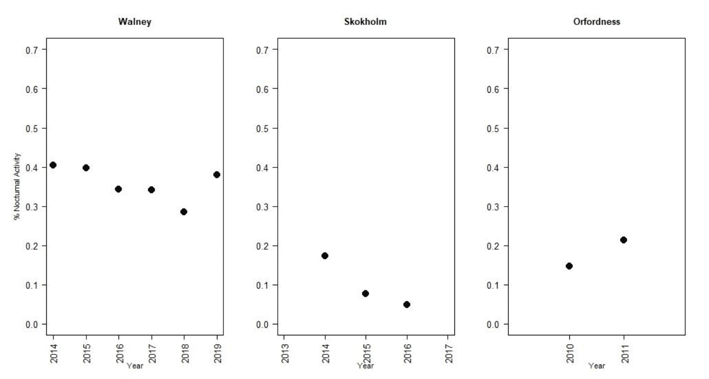
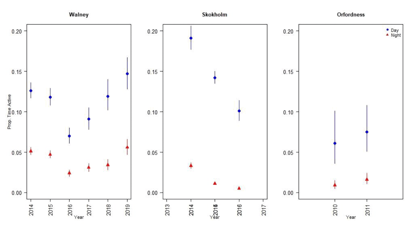
Nocturnal activity levels in lesser black-backed gulls were assessed using data from UvA GPS tags deployed across the breeding season as a whole at Walney, Skokholm and Orfordness (Figure 4). There was substantial variation in activity levels both between years and between colonies. Nocturnal activity levels were greatest at Walney, where they ranged from 28 – 40% of daytime activity, and lowest at Skokholm, where they ranged from 5 – 17% of daytime activity (Tables 2-4). This in part reflects differences in daytime activity levels between colonies, potentially as a result of differences in foraging behaviour between colonies. Whilst birds were active for less than 5% of the time at night, birds were active for 6-19% of the time during the day (Figure 5).
In contrast to gannets and kittiwakes, the attachment methodology used for lesser black-backed gulls meant data were collected across the breeding season as a whole. However, there were no clear trends in nocturnal activity over the course of the breeding season.
| Year | Month | Dawn | Day | Dusk | Night | Nocturnal activity |
|---|---|---|---|---|---|---|
| 2014 | All | 0.19 (0.17 - 0.21) | 0.13 (0.12 - 0.14) | 0.11 (0.10 - 0.118) | 0.05 (0.05 - 0.056) | 0.41 (0.40 - 0.41) |
| 5 | 0.07 (0.06 - 0.09) | 0.05 (0.04 - 0.06) | 0.04 (0.03 - 0.05) | 0.03 (0.02 - 0.03) | 0.48 (0.47 - 0.49) | |
| 6 | 0.21 (0.18 - 0.23) | 0.15 (0.14 - 0.16) | 0.10 (0.09 - 0.12) | 0.04 (0.04 - 0.05) | 0.28 (0.27 - 0.29) | |
| 7 | 0.22 (0.2-0 - 0.25) | 0.14 (0.12 - 0.14) | 0.16 (0.14 - 0.18) | 0.08 (0.07 - 0.09) | 0.57 (0.56 - 0.58) | |
| 8 | 0.22 (0.16 - 0.30) | 0.10 (0.07 - 0.13) | 0.11 (0.07 - 0.16) | 0.05 (0.04 - 0.07) | 0.52 (0.50 - 0.54) | |
| 2015 | All | 0.236 (0.216 - 0.258) | 0.12 (0.11 - 0.13) | 0.09 (0.08 - 0.11) | 0.05 (0.04 - 0.05) | 0.40 (0.39 - 0.40) |
| 3 | 0.043 (0.02 - 0.10) | 0.03(0.01 - 0.07) | 0.01 (0.00- 0.03) | 0.02 (0.01 - 0.05) | 0.61 (0.60 - 0.62) | |
| 4 | 0.08 (0.06 - 0.11) | 0.05 (0.04 - 0.07) | 0.02 (0.02 - 0.03) | 0.03 (0.03 - 0.04) | 0.63 (0.62 - 0.64) | |
| 5 | 0.16 (0.14 - 0.19) | 0.09 (0.08 - 0.10) | 0.06 (0.05 - 0.07) | 0.01 (0.01 - 0.01) | 0.13 (0.12 - 0.13) | |
| 6 | 0.28 (0.25 - 0.31) | 0.14 (0.13 - 0.16) | 0.11 (0.10 - 0.131) | 0.04 (0.04 - 0.05) | 0.28 (0.27 - 0.29) | |
| 7 | 0.36 (0.32 - 0.39) | 0.14 (0.13 - 0.16) | 0.18 (0.16 - 0.21) | 0.11 (0.10 - 0.12) | 0.78 (0.77 - 0.79) | |
| 2016 | All | 0.12 (0.10 - 0.14) | 0.07 (0.06 - 0.08) | 0.05 (0.04 - 0.06) | 0.02 (0.02 - 0.03) | 0.34 (0.34 - 0.34) |
| 5 | 0.13 (0.10 - 0.16) | 0.07 (0.06 - 0.09) | 0.05 (0.04 - 0.07) | 0.02 (0.02 - 0.03) | 0.28 (0.28 - 0.29) | |
| 6 | 0.12 (0.10 - 0.15) | 0.07 (0.06 - 0.09) | 0.06 (0.05 - 0.08) | 0.03 (0.02 - 0.03) | 0.38 (0.37 - 0.38) | |
| 7 | 0.03 (0.02 - 0.04) | 0.01(0.01 - 0.02) | 0.01 (0.00 - 0.01) | 0.01 (0.00 - 0.01) | 0.42 (0.41 - 0.42) | |
| 2017 | All | 0.16 (0.14 - 0.19) | 0.09 (0.08 - 0.11) | 0.08 (0.07 - 0.09) | 0.03 (0.03 - 0.04) | 0.34 (0.34 - 0.35) |
| 4 | 0.08 (0.05 - 0.12) | 0.05 (0.03 - 0.08) | 0.04 (0.02 - 0.06) | 0.01 (0.01 - 0.02) | 0.25 (0.25 - 0.26) | |
| 5 | 0.14 (0.12 - 0.16) | 0.08 (0.07 - 0.093) | 0.05 (0.04 - 0.07) | 0.02 (0.02 - 0.03) | 0.29 (0.28 - 0.29) | |
| 6 | 0.22 (0.19 - 0.26) | 0.11 (0.10 - 0.13) | 0.13 (0.11 - 0.16) | 0.06 (0.05 - 0.07) | 0.50 (0.48 - 0.51) | |
| 8 | 0.14 (0.12 - 0.19) | 0.09 (0.07 - 0.12) | 0.07 (0.05 - 0.10) | 0.03 (0.02 - 0.04) | 0.28 (0.27 - 0.30) | |
| 2018 | All | 0.19 (0.16 - 0.22) | 0.12 (0.10 - 0.14) | 0.09 (0.07 - 0.11) | 0.03 (0.03 - 0.04) | 0.29 (0.28 - 0.29) |
| 5 | 0.14 (0.10 - 0.19) | 0.09 (0.07 - 0.12) | 0.07 (0.05 - 0.10) | 0.03 (0.02 - 0.04) | 0.28 (0.27 - 0.30) | |
| 6 | 0.25 (0.21 - 0.30) | 0.17(0.14 - 0.20) | 0.12 (0.09 - 0.15) | 0.05 (0.04 - 0.07) | 0.31 (0.29 - 0.32) | |
| 7 | 0.50 (0.43 - 0.57) | 0.33 (0.31 - 0.35) | 0.14 (0.09 - 0.20) | 0.05 (0.04 - 0.07) | 0.15 (0.12 - 0.19) | |
| 2019 | All | 0.28 (0.24 - 0.33) | 0.15 (0.13 - 0.17) | 0.12 (0.105 - 0.15) | 0.06 (0.05 - 0.07) | 0.38 (0.37 - 0.39) |
| 5 | 0.25 (0.20 - 0.31) | 0.15 (0.13 - 0.18) | 0.13 (0.10 - 0.16) | 0.05 (0.04 - 0.06) | 0.34 (0.32 - 0.35) | |
| 6 | 0.32 (0.26 - 0.39) | 0.12 (0.10 - 0.15) | 0.10(0.07 - 0.14) | 0.06 (0.05 - 0.08) | 0.49 (0.46 - 0.52) |
| Year | Month | Dawn | Day | Dusk | Night | Nocturnal activity |
|---|---|---|---|---|---|---|
| 2014 | All | 0.21 (0.19 - 0.23) | 0.19(0.18 - 0.21) | 0.13 (0.12 - 0.15) | 0.03 (0.03 - 0.04) | 0.17 (0.17 - 0.18) |
| 5 | 0.15 (0.13 - 0.18) | 0.14 (0.13 - 0.15) | 0.09 (0.08 - 0.11) | 0.01 (0.01 - 0.01) | 0.08 (0.07 - 0.08) | |
| 6 | 0.28 (0.25 - 0.32) | 0.24 (0.22 - 0.27) | 0.17 (0.15 - 0.19) | 0.05 (0.04 - 0.06) | 0.21 (0.20 - 0.22) | |
| 7 | 0.11 (0.10 - 0.13) | 0.14 (0.13 - 0.15) | 0.09 (0.08 - 0.11) | 0.03 (0.03 - 0.03) | 0.21 (0.21 - 0.22) | |
| 8 | 0.11 (0.08 - 0.16) | 0.14 (0.11 - 0.17) | 0.08 (0.05 - 0.11) | 0.02 (0.01- 0.02) | 0.11 (0.10 - 0.12) | |
| 2015 | All | 0.18 (0.17 - 0.19) | 0.14 (0.14 - 0.15) | 0.10 (0.09 - 0.11) | 0.01 (0.01 - 0.01) | 0.07 (0.07 - 0.08) |
| 5 | 0.13 (0.11 - 0.15) | 0.12 (0.11 - 0.13) | 0.09 (0.08 - 0.11) | 0.01 (0.01 - 0.01) | 0.07 (0.06 - 0.07) | |
| 6 | 0.26 (0.23 - 0.30) | 0.17 (0.15 - 0.20) | 0.16 (0.14 - 0.19) | 0.04 (0.03 - 0.04) | 0.21 (0.20 - 0.22) | |
| 7 | 0.20 (0.18 - 0.23) | 0.16 (0.15 - 0.18) | 0.14 (0.12 - 0.17) | 0.02 (0.01 - 0.02) | 0.10 (0.01 - 0.11) | |
| 2016 | All | 0.10 (0.09 - 0.12) | 0.10 (0.09 - 0.11) | 0.07 (0.06 - 0.09) | 0.01 (0.00 - 0.01) | 0.05 (0.05 - 0.05) |
| 5 | 0.16 (0.13 - 0.19) | 0.15 (0.13 - 0.16) | 0.14 (0.12 - 0.17) | 0.0216 (0.01 - 0.02) | 0.11 (0.01 - 0.11) | |
| 6 | 0.21 (0.18 - 0.26) | 0.15 (0.13 - 0.17) | 0.18 (0.15 - 0.23) | 0.02 (0.02 - 0.03) | 0.16 (0.15 - 0.18) |
| Year | Month | Dawn | Day | Dusk | Night | Nocturnal activity |
|---|---|---|---|---|---|---|
| 2010 | All | 0.06 (0.04 - 0.11) | 0.06 (0.04 - 0.10) | 0.04 (0.022 - 0.07) | 0.01 (0.01 - 0.02) | 0.14 (0.14 - 0.15) |
| 6 | 0.05 (0.02 - 0.09) | 0.04 (0.02 - 0.08) | 0.03 (0.01 - 0.06) | 0.01 (0.00 - 0.01) | 0.15 (0.14 - 0.15) | |
| 7 | 0.14 (0.10 - 0.21) | 0.16 (0.12 - 0.20) | 0.08 (0.05 - 0.13) | 0.02 (0.01 - 0.03) | 0.13 (0.12 - 0.16) | |
| 2011 | All | 0.09 (0.07 - 0.14) | 0.08 (0.05 - 0.11) | 0.05 (0.03 - 0.07) | 0.02 (0.01 - 0.02) | 0.22 (0.21 - 0.22) |
| 5 | 0.04 (0.03 - 0.05) | 0.04 (0.03 - 0.06) | 0.03 (0.02 - 0.04) | 0.01 (0.01 - 0.01) | 0.20 (0.19 - 0.20) | |
| 6 | 0.13 (0.09 - 0.19) | 0.11 (0.08 - 0.16) | 0.08 (0.05 - 0.11) | 0.03 (0.02 - 0.04) | 0.23 (0.22 - 0.24) | |
| 7 | 0.12 (0.08 - 0.18) | 0.07 (0.05 - 0.10) | 0.04 (0.03 - 0.07) | 0.01 (0.01 - 0.02) | 0.20 (0.19 - 0.21) |
3.1.2. Kittiwake
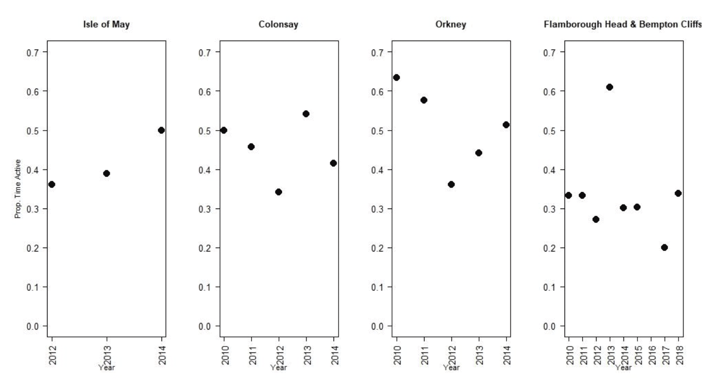
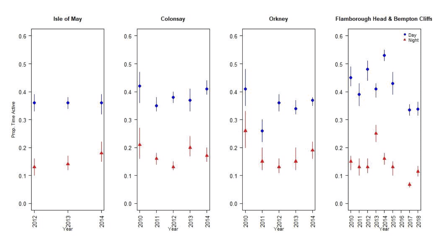
Nocturnal activity in kittiwakes was collected using IGotU GPS tags deployed on birds at Colonsay, Isle of May, Orkney, Flamborough Head and Bempton Cliffs, and from UvA tags deployed birds at Flamborough Head and Bempton Cliffs. Levels of nocturnal activity showed substantial variation between colonies and years, from 27 – 63 % of daytime activity (Figure 6, Tables 5 & 6). However, understanding these differences is challenging due to the different tag types used. The longer-term deployment of the UvA tags means it is possible to get a clearer picture of nocturnal activity over the breeding season as a whole, in comparison to the IGotU tags which were shorter term deployments, typically focussed on the period around early chick rearing. Possibly reflecting this, overall activity levels estimated from the UvA tags were lower than those estimated using IGotU tags (Figure 7). However, estimates of nocturnal activity as a proportion of daytime activity obtained from UvA tags also showed variation between years, at 20% in 2017 and 33% in 2018 (Table 6).
| Site | Year | Dawn | Day | Dusk | Night | Nocturnal Activity |
|---|---|---|---|---|---|---|
| Isle of May | 2012 | 0.10 (0.06 - 0.16) | 0.36 (0.33 - 0.39) | 0.29 (0.22 - 0.38) | 0.13 (0.1 - 0.16) | 0.36 (0.30 – 0.41) |
| 2013 | 0.2 (0.15 - 0.26) | 0.36 (0.34 - 0.38) | 0.42 (0.35 - 0.48) | 0.14 (0.12 - 0.17) | 0.38 (0.35 – 0.45) | |
| 2014 | 0.06 (0.03 - 0.11) | 0.36 (0.32 - 0.39) | 0.41 (0.32 - 0.50) | 0.18 (0.15 - 0.22) | 0.5 (0.46 – 0.56) | |
| Flamborough Head and Bempton Cliffs | 2010 | 0.21 (0.15 - 0.28) | 0.45 (0.42 - 0.49) | 0.45 (0.38 - 0.53) | 0.15 (0.12 - 0.17) | 0.33 (0.28 – 0.34) |
| 2011 | 0.17 (0.11 - 0.25) | 0.39 (0.35 - 0.43) | 0.26 (0.18 - 0.35) | 0.13 (0.1 - 0.16) | 0.33 (0.28 – 0.37) | |
| 2012 | 0.15 (0.1 - 0.22) | 0.48 (0.44 - 0.51) | 0.45 (0.36 - 0.54) | 0.13 (0.11 - 0.16) | 0.27 (0.25 – 0.31) | |
| 2013 | 0.22 (0.16 - 0.29) | 0.41 (0.38 - 0.43) | 0.43 (0.36 - 0.51) | 0.25 (0.22 - 0.28) | 0.61 (0.57 – 0.65) | |
| 2014 | 0.21 (0.16 - 0.27) | 0.53 (0.51 - 0.55) | 0.33 (0.27 - 0.38) | 0.16 (0.14 - 0.18) | 0.30 (0.27 – 0.32) | |
| 2015 | 0.22 (0.16 - 0.30) | 0.43 (0.39 - 0.47) | 0.37 (0.29 - 0.46) | 0.13 (0.1 - 0.15) | 0.30 (0.25 – 0.32) | |
| Colonsay | 2010 | 0.28 (0.17 - 0.42) | 0.42 (0.36 - 0.47) | 0.58 (0.44 - 0.7) | 0.21 (0.16 - 0.27) | 0.5 (0.44 – 0.57) |
| 2011 | 0.17 (0.13 - 0.22) | 0.35 (0.33 - 0.38) | 0.35 (0.29 - 0.4) | 0.16 (0.14 - 0.18) | 0.45 (0.42 – 0.47) | |
| 2012 | 0.21 (0.17 - 0.25) | 0.38 (0.36 - 0.4) | 0.35 (0.3 - 0.39) | 0.13 (0.12 - 0.15) | 0.34 (0.33 – 0.37) | |
| 2013 | 0.23 (0.17 - 0.31) | 0.37 (0.33 - 0.41) | 0.44 (0.35 - 0.52) | 0.2 (0.17 - 0.24) | 0.54 (0.51 – 0.58) | |
| 2014 | 0.23 (0.17 - 0.30) | 0.41 (0.39 - 0.44) | 0.42 (0.34 - 0.49) | 0.17 (0.15 - 0.20) | 0.41 (0.38 – 0.45) | |
| Orkney | 2010 | 0.37 (0.28 - 0.48) | 0.41 (0.35 - 0.48) | 0.34 (0.25 - 0.44) | 0.26 (0.2 - 0.33) | 0.63 (0.57 – 0.68) |
| 2011 | 0.2 (0.14 - 0.26) | 0.26 (0.22 - 0.3) | 0.19 (0.14 - 0.26) | 0.15 (0.12 - 0.2) | 0.57 (0.54 – 0.66) | |
| 2012 | 0.11 (0.08 - 0.15) | 0.36 (0.33 - 0.39) | 0.3 (0.26 - 0.35) | 0.13 (0.11 - 0.16) | 0.36 (0.33 – 0.41) | |
| 2013 | 0.25 (0.17 - 0.36) | 0.34 (0.32 - 0.37) | 0.35 (0.26 - 0.45) | 0.15 (0.12 - 0.2) | 0.44 (0.37 – 0.54) | |
| 2014 | 0.13 (0.09 - 0.19) | 0.37 (0.35 - 0.38) | 0.32 (0.25 - 0.38) | 0.19 (0.16 - 0.22) | 0.51 (0.45 – 0.57) |
| Year | Month | Dawn | Day | Dusk | Night | Nocturnal activity |
|---|---|---|---|---|---|---|
| 2017 | All | 0.38 (0.34 – 0.4326) | 0.34 (0.32 – 0.35) | 0.17 (0.14 – 0.20) | 0.07 (0.06 – 0.08) | 0.20 (0.19 – 0.21) |
| June | 0.40 (0.34 – 0.46) | 0.33 (0.31 – 0.35) | 0.20 (0.16 – 0.24) | 0.07 (0.06 – 0.08) | 0.22 (0.19 – 0.24) | |
| July | 0.36 (0.30 – 0.42) | 0.34 (0.31 – 0.37) | 0.10 (0.07 – 0.14) | 0.06 (0.48 – 0.07) | 0.17 (0.16 – 0.20) | |
| 2018 | All | 0.22 (0.17 – 0.28) | 0.34 (0.32 – 0.36) | 0.31 (0.27 – 0.36) | 0.11 (0.10 – 0.13) | 0.34 (0.31 – 0.37) |
| June | 0.11 (0.05 – 0.25) | 0.28 (0.25 – 0.30) | 0.20 (0.13 – 0.30) | 0.10 (0.07 – 0.13) | 0.35 (0.30 – 0.44) | |
| July | 0.26 (0.19 – 0.33) | 0.36 (0.34 – 0.39) | 0.35 (0.30 – 0.41) | 0.12 (0.10 - 0.15) | 0.34 (0.30 – 0.37) |
3.1.3. Gannet
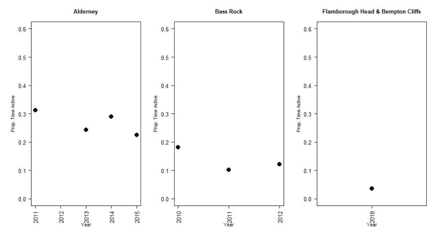
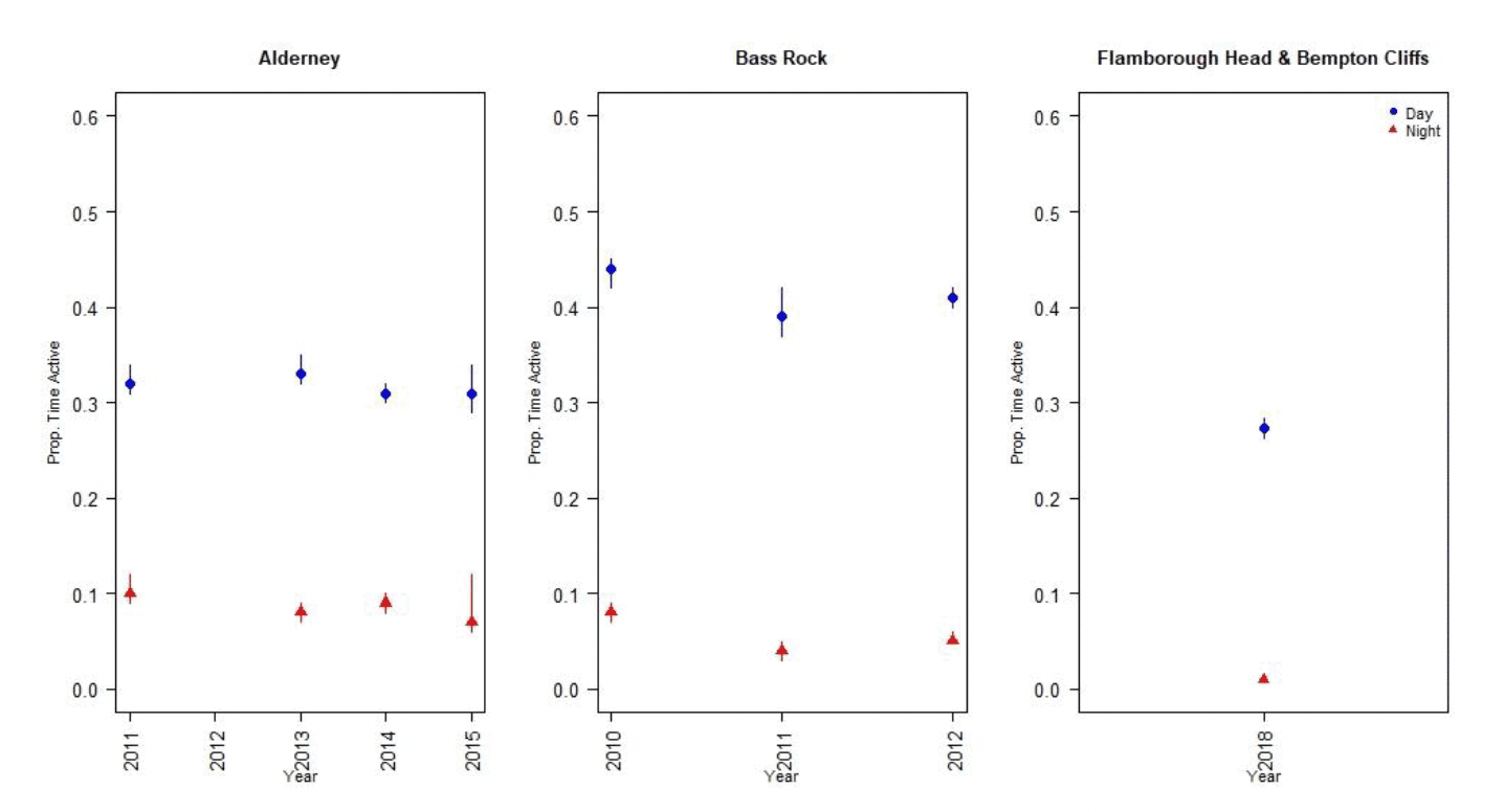
Nocturnal activity in gannets was collected using IGotU GPS tags deployed on birds at the Bass Rock and Alderney, and from UvA tags deployed birds at Flamborough Head and Bempton Cliffs. Levels of nocturnal activity showed substantial variation between colonies and years, from 4 – 31 % of daytime activity (Figure 8, Tables 7 & 8). However, understanding these differences is challenging due to the different tag types used. The longer-term deployment of the UvA tags means it is possible to get a clearer picture of nocturnal activity over the breeding season as whole, in comparison to the IGotU tags which were shorter term deployments, typically focussed on the period around early chick rearing. This may be reflected in the lower levels of activity estimated at night for birds from Flamborough Head and Bempton Cliffs (Figure 9).
| Site | Year | Dawn | Day | Dusk | Night | Nocturnal Activity |
|---|---|---|---|---|---|---|
| Alderney | 2011 | 0.08 (0.05 – 0.12) | 0.32 (0.31- 0.34) | 0.31 (0.26 – 0.37) | 0.1 (0.09-0.12) | 0.31 (0.29 – 0.35) |
| 2013 | 0.31 (0.27 - 0.36) | 0.33 (0.32 - 0.35) | 0.23 (0.2 - 0.27) | 0.08 (0.07 - 0.09) | 0.24 (0.22 – 0.26) | |
| 2014 | 0.51 (0.46 - 0.56) | 0.31 (0.3 - 0.32) | 0.4 (0.36 - 0.45) | 0.09 (0.08 - 0.1) | 0.29 (0.27 – 0.31) | |
| 2015 | 0.06 (0.04 - 0.12) | 0.31 (0.29 - 0.34) | 0.29 (0.26 - 0.37) | 0.07 (0.06 - 0.12) | 0.22 (0.2 – 0.35) | |
| Bass Rock | 2010 | 0.13 (0.1 - 0.16) | 0.44 (0.42 - 0.45) | 0.45 (0.41 - 0.49) | 0.08 (0.07 - 0.09) | 0.18 (0.16 – 0.2) |
| 2011 | 0.36 (0.32 - 0.4) | 0.39 (0.37 - 0.42) | 0.26 (0.22 - 0.3) | 0.04 (0.03 - 0.05) | 0.10 (0.08 – 0.12) | |
| 2012 | 0.43 (0.39 - 0.46) | 0.41 (0.4 - 0.42) | 0.21 (0.19 - 0.24) | 0.05 (0.05 - 0.06) | 0.13 (0.12 – 0.14) | |
| 2015 | 0.35 (0.31 - 0.15) | 0.42 (0.4 - 0.45) | 0.22 (0.19 - 0.49) | 0.03 (0.03 - 0.09) | 0.07 (0.07 – 0.2) |
| Month | Dawn | Day | Dusk | Night | Nocturnal activity |
|---|---|---|---|---|---|
| All | 0.19 (0.17-0.22) | 0.27 (0.26 – 0.28) | 0.21 (0.19 – 0.23) | 0.01 (0.01 – 0.01) | 0.04 (0.03 – 0.05) |
| July | 0.13 (0.10 – 0.17) | 0.26 (0.25 – 0.27) | 0.19 (0.16 – 0.22) | 0.01 (0.01 0.02) | 0.05 (0.04 – 0.06) |
| August | 0.27 (0.22 – 0.33) | 0.31 (0.28 – 0.33) | 0.27 (0.23 – 0.32) | 0.01 (0.01 – 0.02) | 0.05 (0.048 – 0.05) |
| September | 0.20 (0.15 – 0.28) | 0.24 (0.22 – 0.26) | 0.12 (0.07 – 0.18) | 0.01 (0.00 – 0.01) | 0.03 (0.01 – 0.04) |
3.2. Flight speed
3.2.1. Autocorrelation assessment
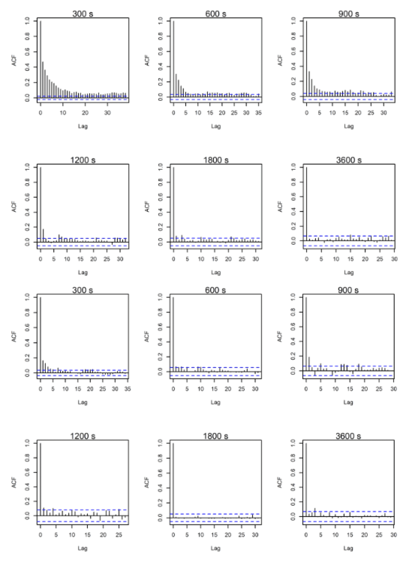
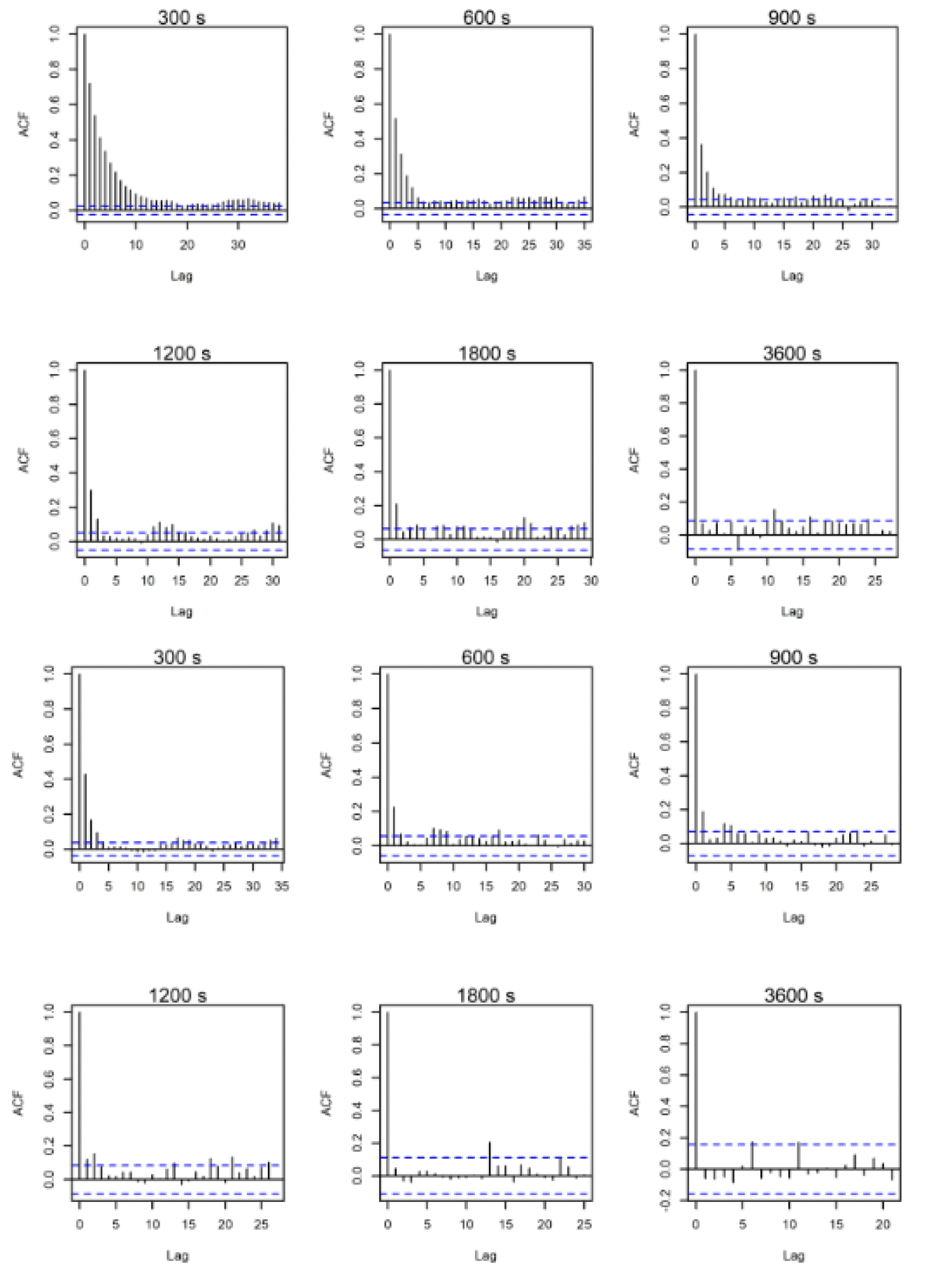
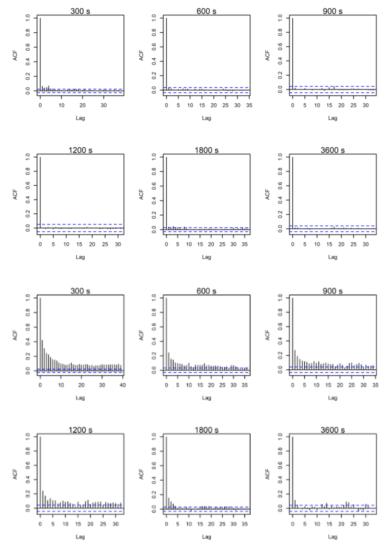
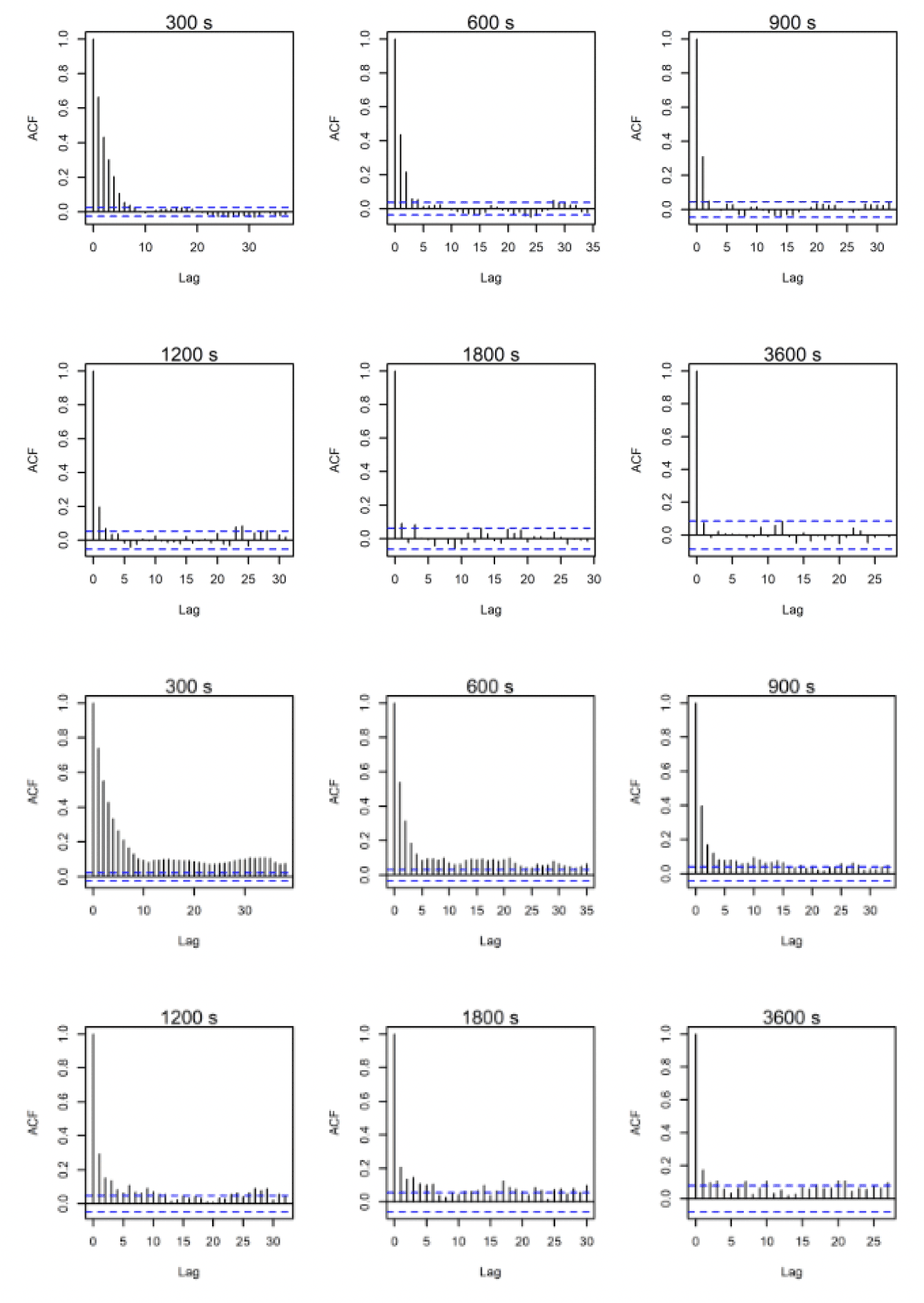
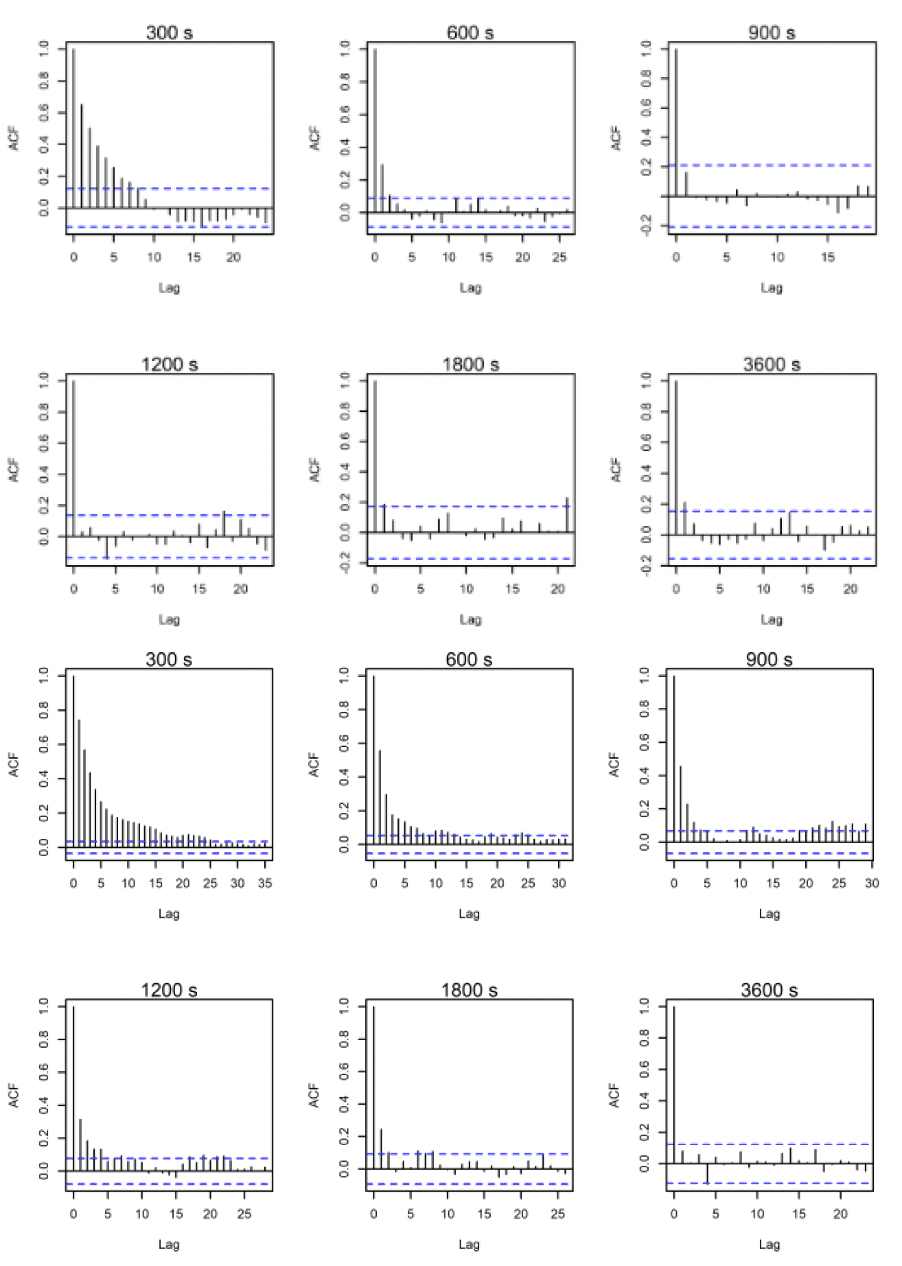
ACF comparisons were carried out for the full dataset including onshore data. Autocorrelation can be assessed visually with reference to an ACF plot (figures 10-12). These plots highlight the significance of any correlation between an estimated flight speed and subsequent estimates of flight speed. The blue lines on these plots indicate significance at p = 0.05 and, ideally, all vertical lines except the first should be between these. Overall, the temporal autocorrelation was very evident in the data at 300s-900s thereafter improving greatly, with best results (i.e., least autocorrelation) at 3,600s (Figs. 10-12). Consequently, the full dataset for all sites was sub-sampled at 3,600s for further comparisons and subsetted for the offshore environment only. An example is shown in figures 10-12 for lesser black-backed gulls from Walney, Skokholm and Orfordness.
(a) Instantaneous speed
(b) Trajectory speed
(a) Instantaneous speed
(b) Trajectory speed
(a) Instantaneous speed
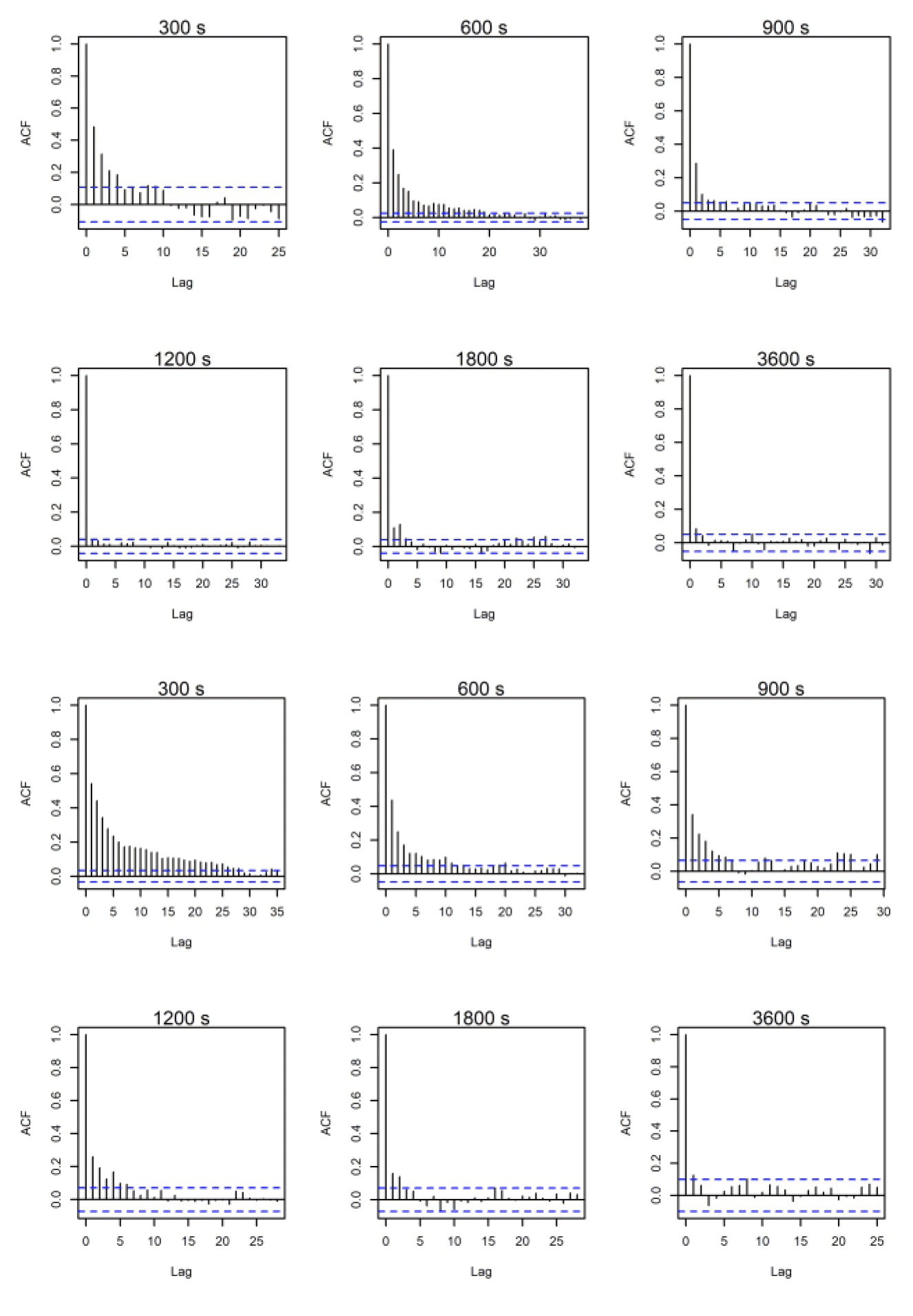
(b) Trajectory speed
3.2.2. Lesser Black-backed Gull Walney
A minimum of five data points were specified for each individual to remove birds with too few data following sub-sampling within the offshore environment at the hourly rate. The resulting offshore dataset was therefore reduced to 1,345 data points for 31 individuals that crossed the offshore environment, from the original offshore dataset at five-minute rates containing 25,432 data points and 37 individuals.
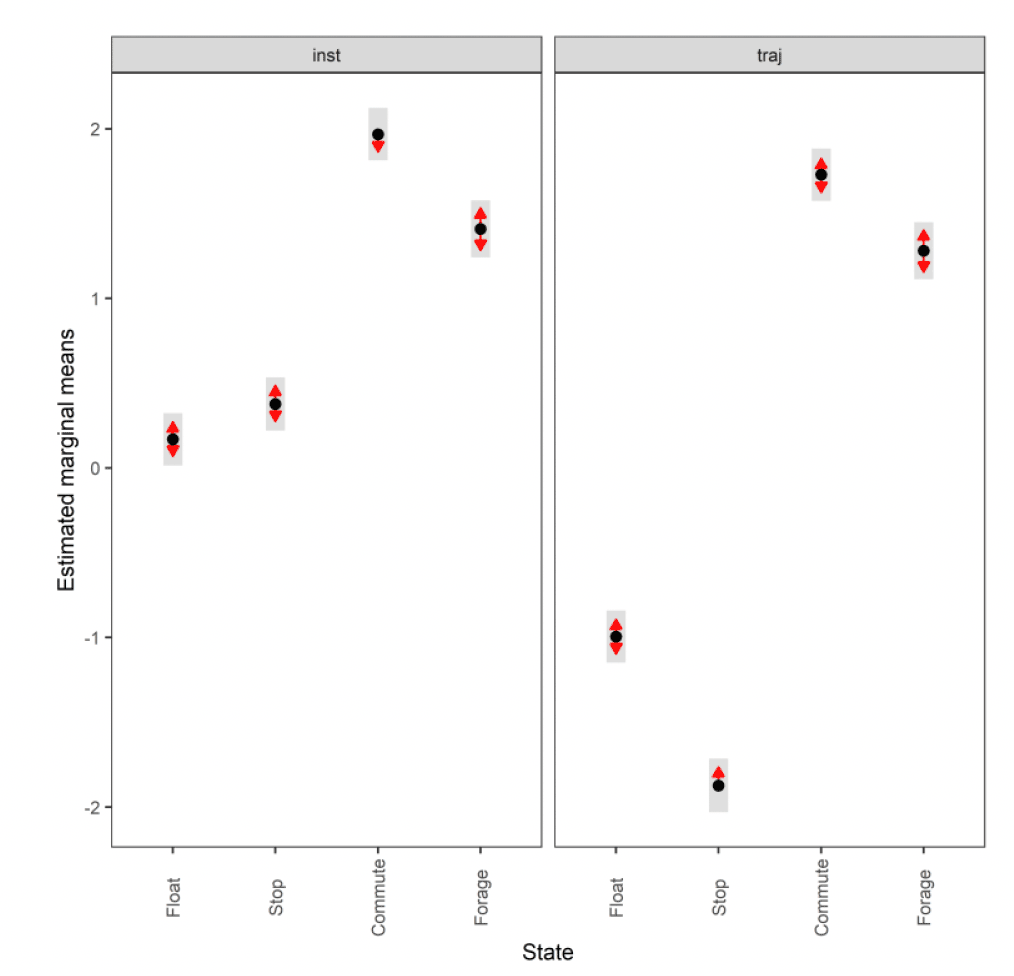
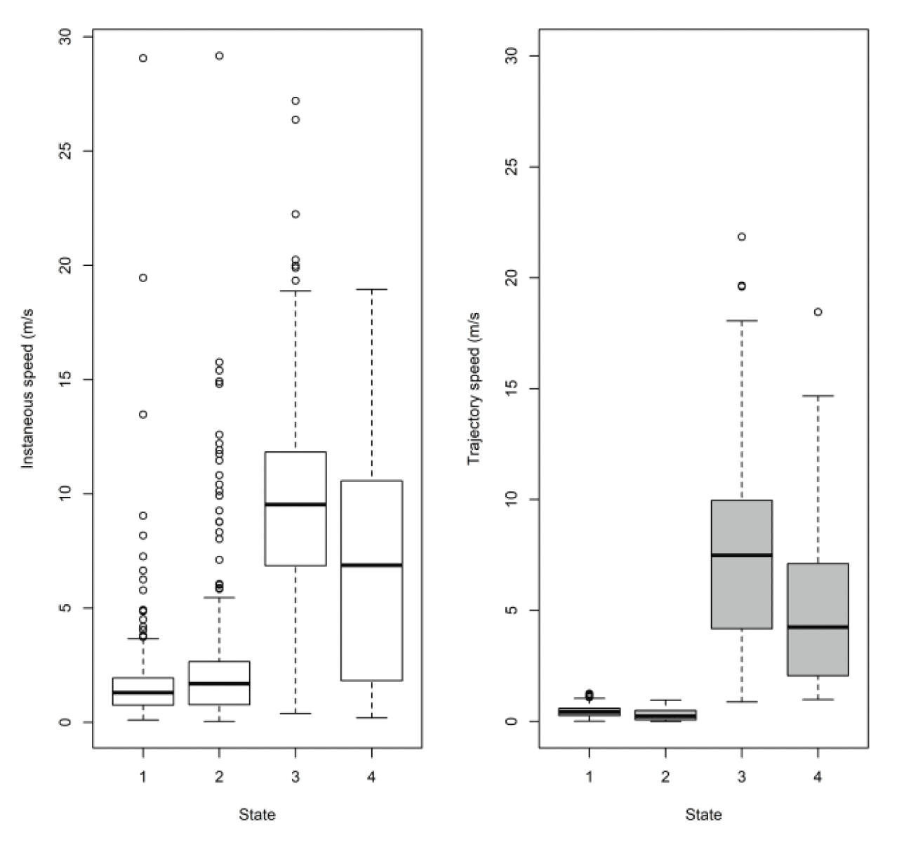
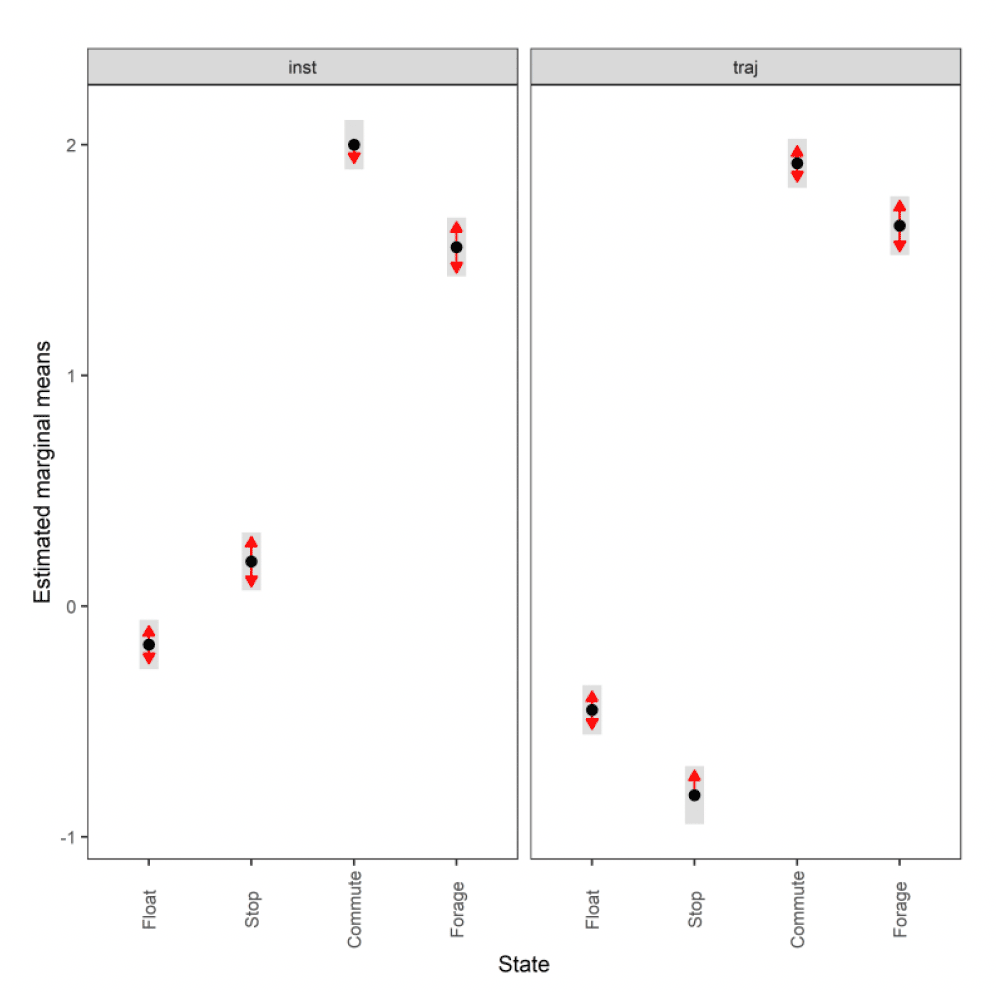
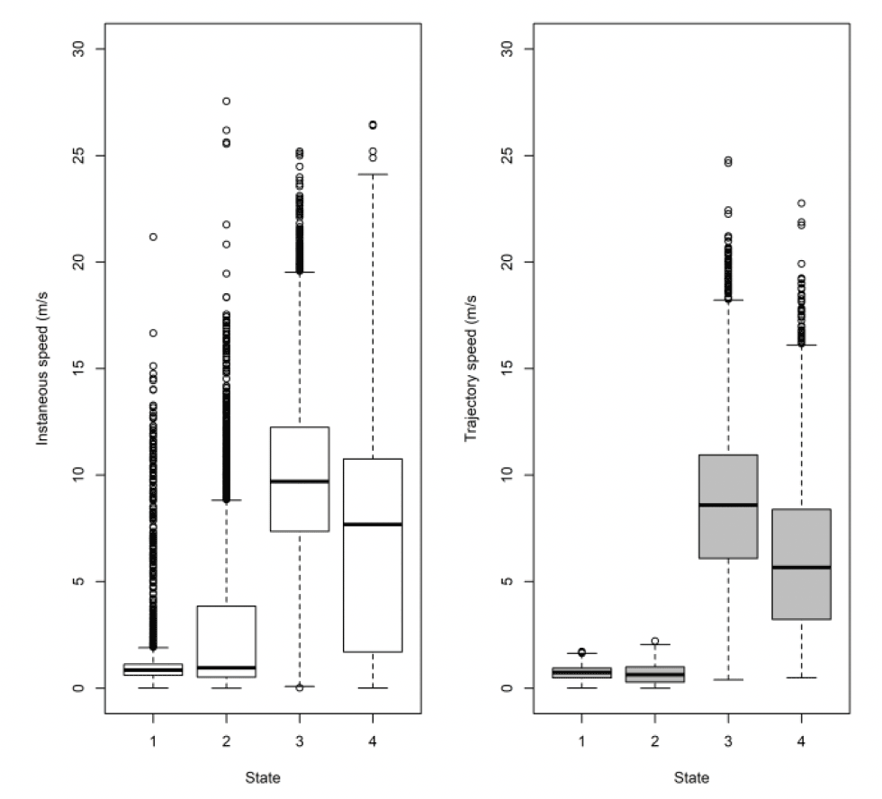
3.2.2.1. Overall statistical comparison between speedsFor South Walney (as was the case at all other colonies), the full GLMM confirmed significantly faster overall speeds offshore than onshore (offshore (1,0) across states: ß = 0.646±0.055, χ2 = 360.61, df = 1, P < 0.001). For Walney offshore movements alone, there was a significant difference between trajectory and instantaneous speeds (χ2 = 312.5, df = 1, P < 0.001) that also varied with state (full two-way interaction: χ2 = 521.52, df = 3, P < 0.001). When assessing the significance of these differences per state through estimated marginal means (Fig 13), there was greatest difference between slower inactive states of stopped and floating on the sea; for commuting (state 3) there was a marginal result with trajectory speed being lower than that of instantaneous, although confidence limits overlapped; for foraging/searching offshore, there was no significant difference between instantaneous and trajectory speeds, although trajectory speeds were again lower than instantaneous. Fastest movements were for commuting for both instantaneous and trajectory speeds.
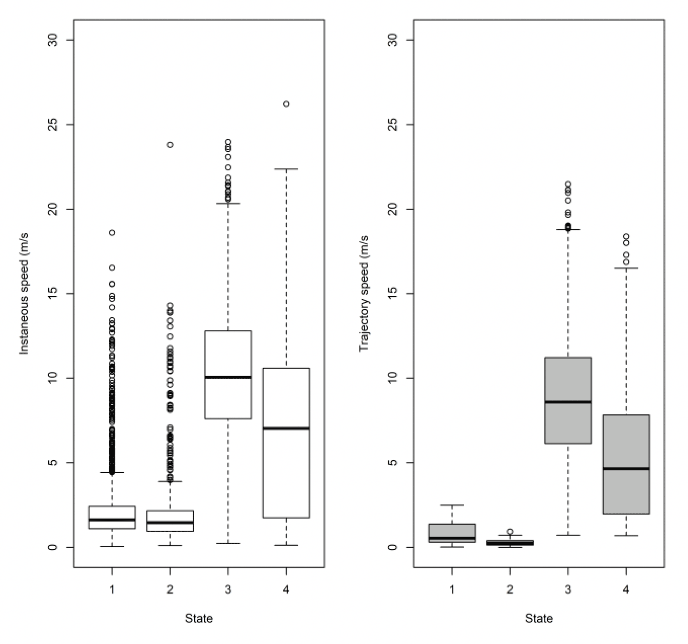
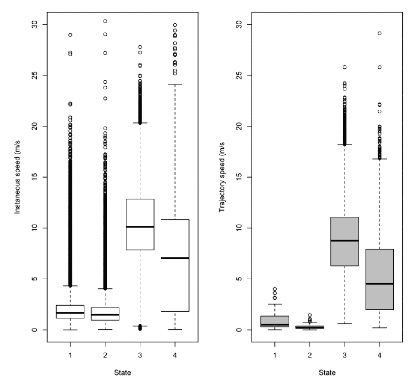
3.2.2.2. Summary of distributions
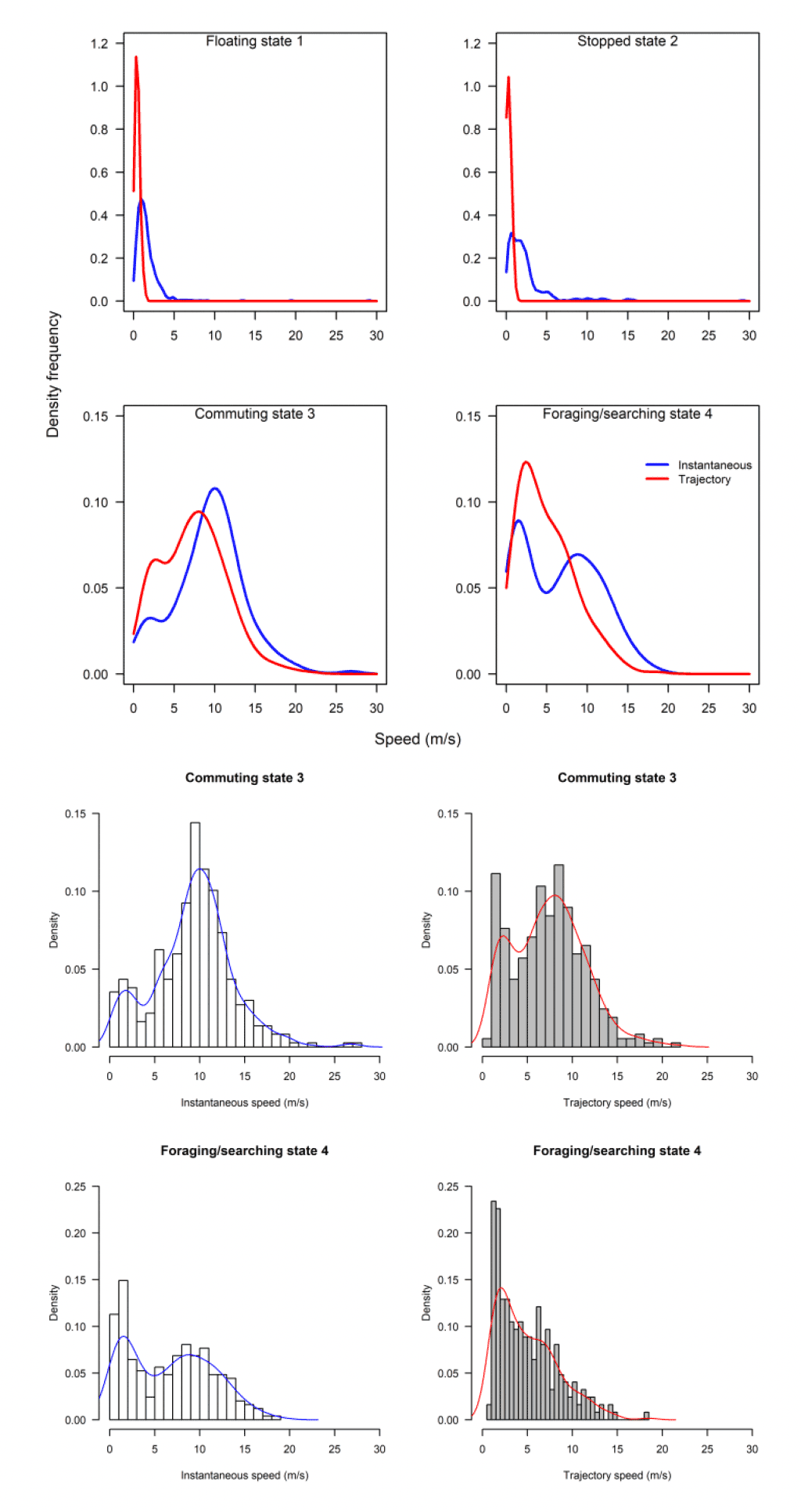
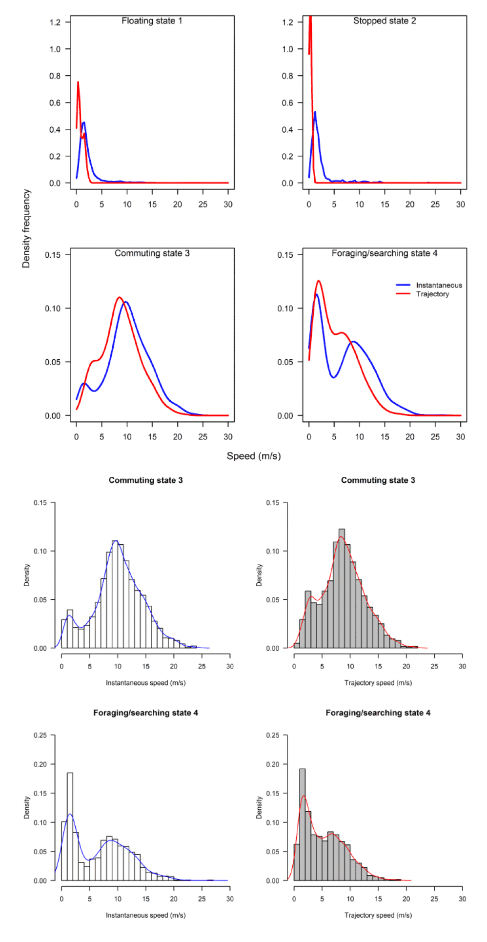
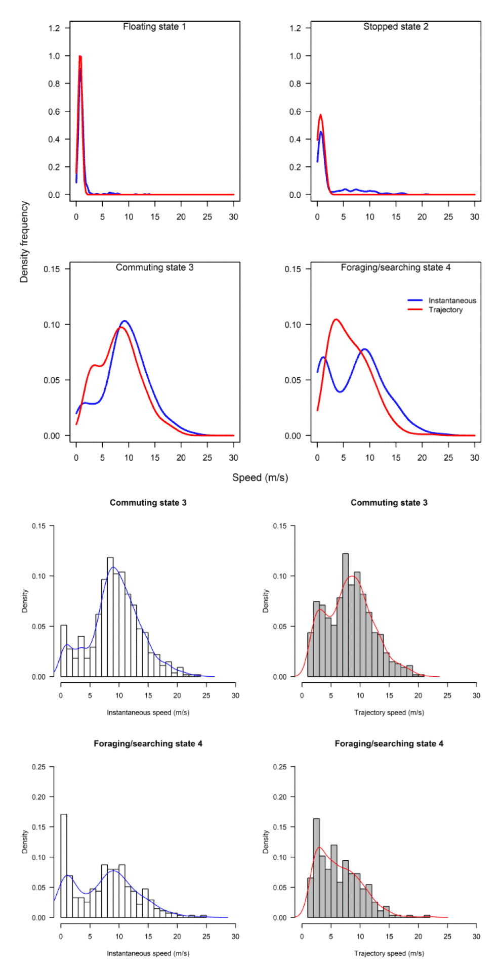
The above analysis by state for each speed type deals with a direct comparison of mean estimates between distributions. However, closer inspection revealed some subtle differences in the distributions that would be overlooked in a direct mean comparison. The distribution of foraging for example, was no different in speed-by-speed type, yet the instantaneous trajectory for Walney showed a double peak in the distribution, one at ca 2 m/s and one at ca 9 m/s, whereas the trajectory speed showed a main peak at about 3 m/s (Fig 14).
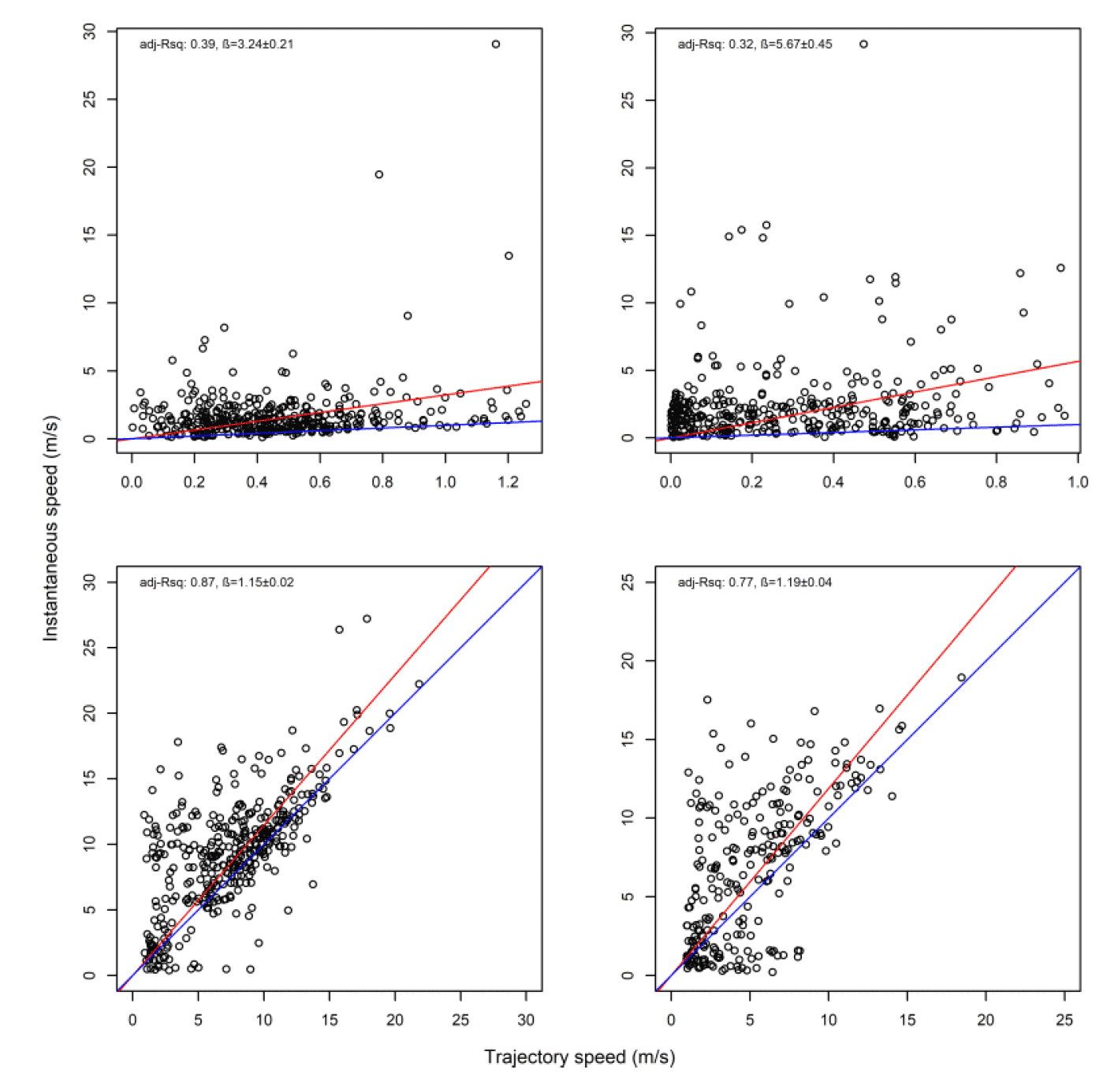
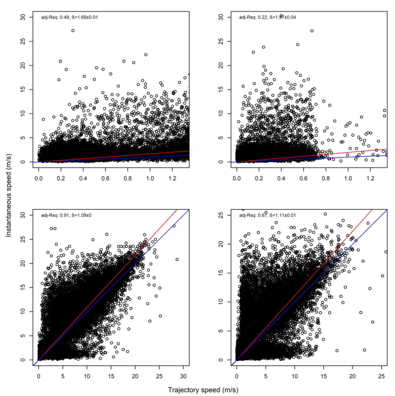
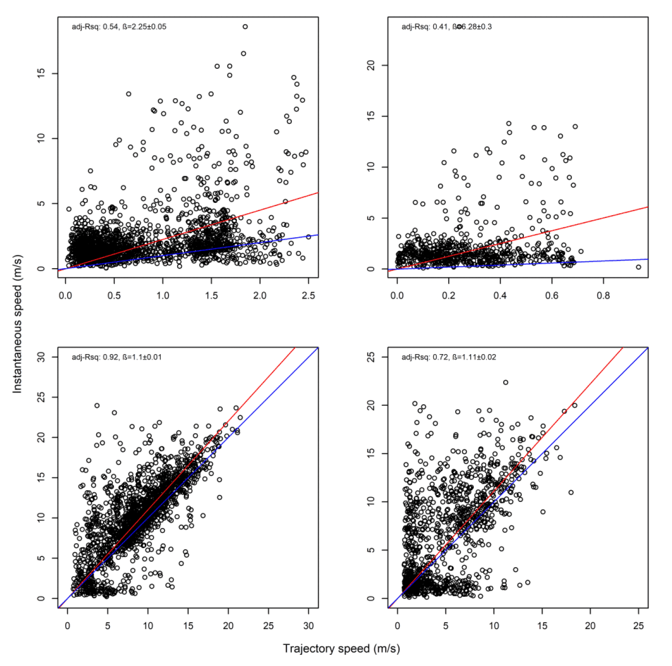
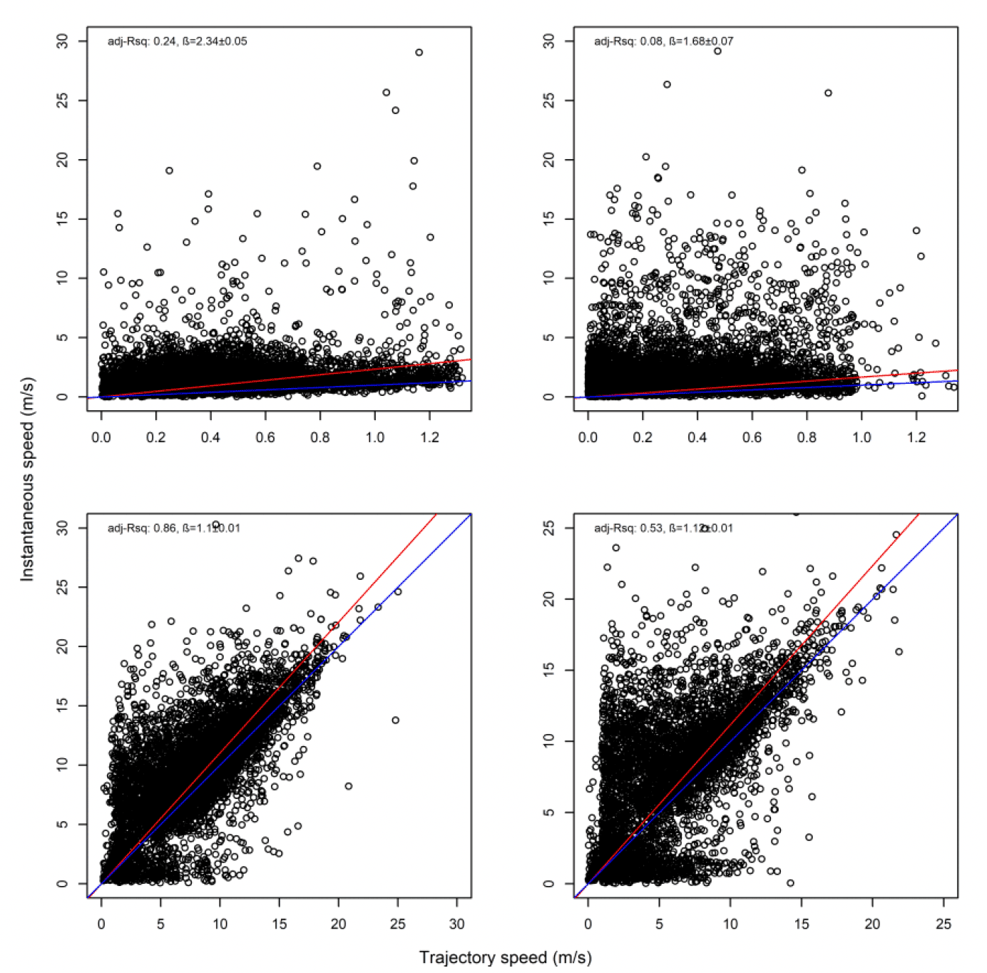
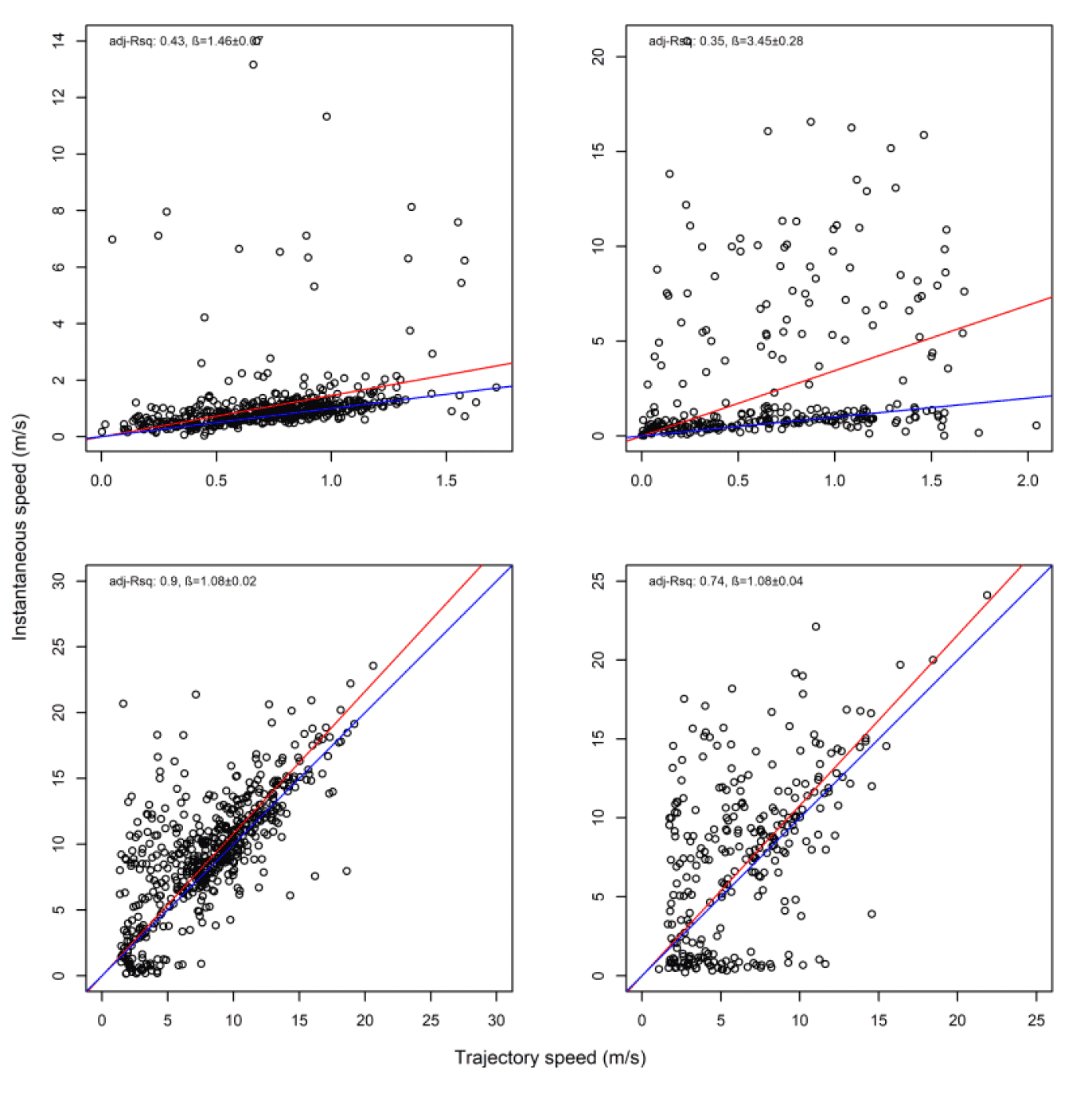
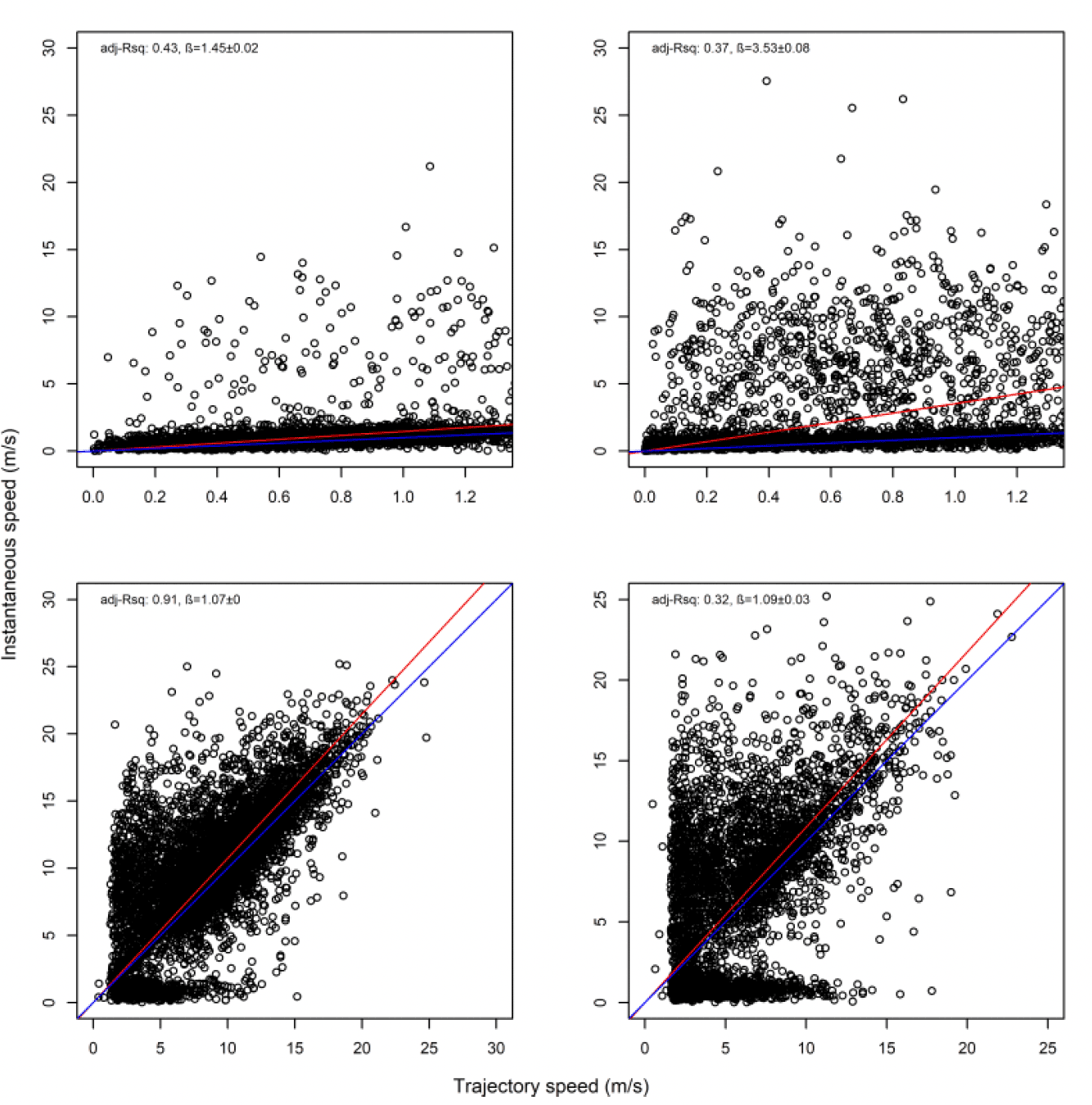
Overall, there was a general bias in underestimating the speed of offshore movement using trajectory speed in comparison to instantaneous velocity (test as above, traj_speed ß = -0.998±0.055 SE, from above full model). These differences were apparent in a direct xy regression (Fig 15), with points biased to the upper left of the 1:1 relationship for all states (as also found by Klaassen et al., 2011 for LBBG during the non-breeding season), and steeper best fit coefficients for commuting and foraging (1.15 and 1.19, respectively). In keeping with the above statistical comparison, the below regressions per state showed much closer relationships for commuting and foraging states than resting ones (Figure 15).
(a) 3600s sub-sample
(b) Original 300s EMbC-classified data
(a) Sub-sample to 1 hour
(b) Original five minute rate
| Colony (n birds) | Data grain | Speed type | 1 (floating) | 2 (stop) | 3 (commuting) | 4 (forage/search) |
|---|---|---|---|---|---|---|
| Walney (n = 33) | 3600s | Instantaneous | 1.30 (0.76,1.94) | 1.69 (0.77,2.66) | 9.53 (6.85,11.82) | 6.87 (1.82,10.57) |
| Trajectory | 0.43 (0.26,0.59) | 0.23 (0.08,0.50) | 7.49 (4.19,9.97) | 4.25 (2.06,7.11) | ||
| Walney (n = 37) | 300s | Instantaneous | 1.32 (0.77,2.05) | 1.51 (0.76,2.61) | 9.51 (7.12,11.88) | 7.94 (2.59,10.79) |
| Trajectory | 0.42 (0.27,0.60) | 0.26 (0.08,0.51) | 8.15 (5.51,10.54) | 5.25 (2.39,8.59) |
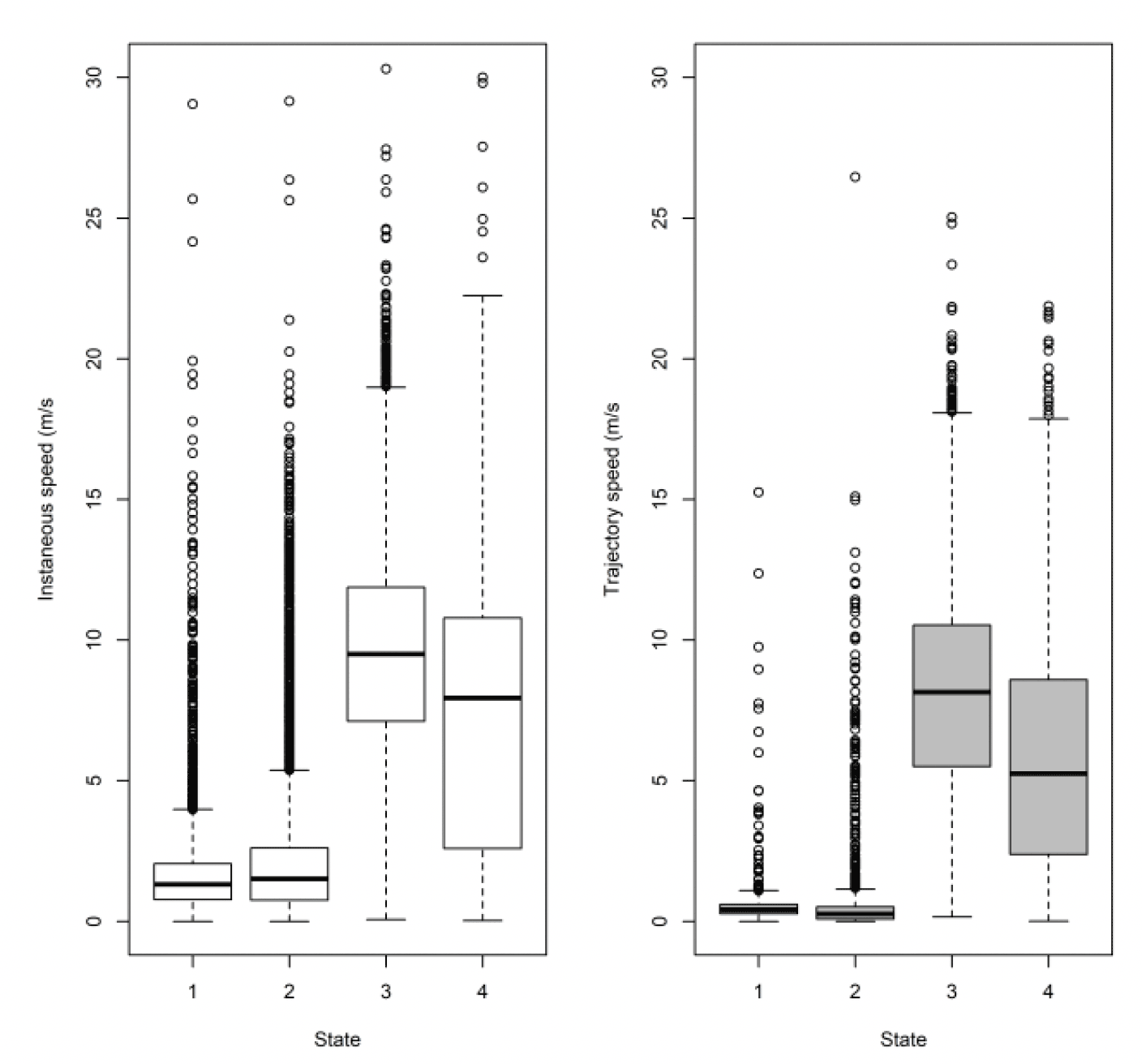
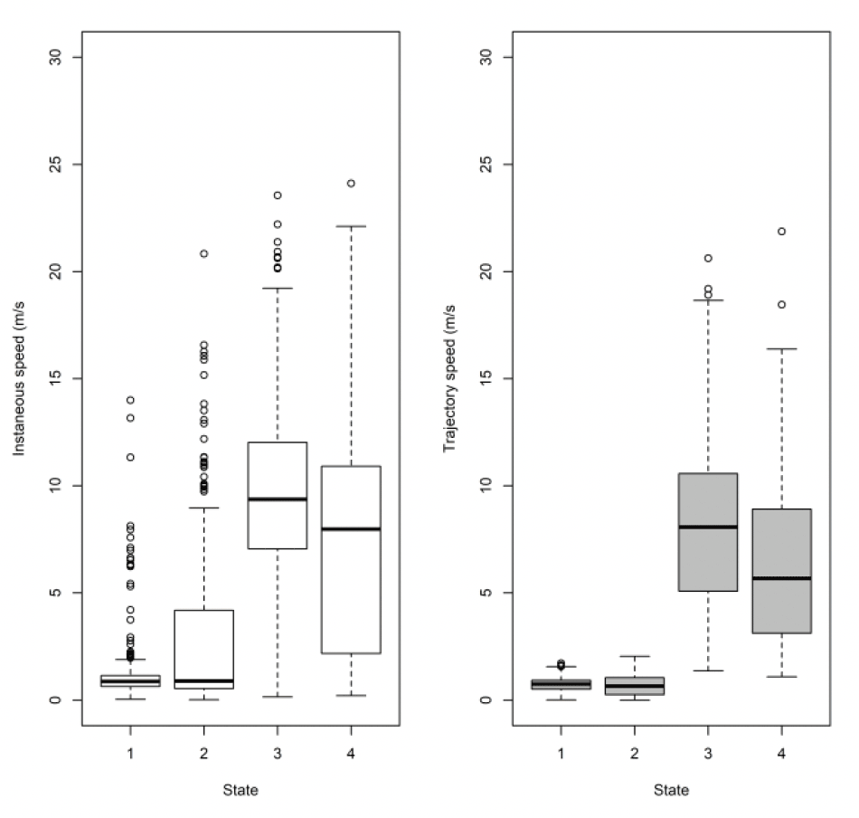
Note, the boxplots above (Figure 16) are based on all the data at five minute rates for comparison to Thaxter et al. (2019). By sub-sampling to hourly rates, we lose about 1 m/s from the commuting mean, so fewer points (and some different birds) meant it was not a fair comparison. Full examination is therefore also required using the 300s data. Comparing to the HMM states, the small steps of states 1 and 2 are comparable. However, the difference lies in where the boundary is drawn between commuting and foraging. EMbC draws the line in a slightly different place, with some foraging points classified as commuting by HMM being classified as foraging by EMbC. This results in slightly different speed distributions by method using the original 300s data. For Thaxter et al. (2019), for example, the median commuting and foraging speeds were 9.2 and 3.6 m/s, whereas for EMBC they are 8.2 and 5.3 m/s.
3.2.3. Lesser Black-backed Gull Skokholm
The original dataset for five-minute rates contained 67,761 rows of offshore data for 24 birds that was further subsampled to 5,486 rows for 24 birds at a rate of 3,600s. Given the offshore location of the colony, no birds were dropped from the analysis in the sub-sampling routine.
3.2.3.1. Overall statistical comparison between speeds
For Skokholm offshore movements, as with Walney, speeds offshore were faster than onshore (ß = 1.882±0.039, P < 0.001) and there was a significant difference between trajectory and instantaneous speeds (χ2 = 676.37 df = 1, P < 0.001) that also varied with state (full two-way interaction: χ2 = 1744.70, df = 3, P < 0.001).
The results for instantaneous vs trajectory speed were the same as for Walney, with the greatest difference between slower inactive states of stopped and floating on the sea and no significant difference for faster states of commuting and foraging.
3.2.3.2. Summary of distributions
As with Walney, closer inspection revealed subtle differences in the distributions. However, comparison of trajectory and instantaneous speeds showed distributions were similar in overall shape (Fig 17). However, there was a general bias in underestimating the speed of offshore movement using trajectory speed in comparison to instantaneous speed (test as above, traj_speed ß = -0.671±0.025 SE, from above full model). As with Walney, these differences were apparent in a direct xy regression (Fig 18), with points biased to the upper left of the 1:1 relationship for all states, and steeper best fit coefficients for commuting and foraging (1.10 and 1.11, respectively). In keeping with the above statistical comparison, the below regression per state showed much closer relationships for commuting and foraging states than resting ones.
(a) 3600s sub-sample
(b) Original 300s EMbC-classified data
(a) sub-sample to 1 hour
(b) Original five minute rate
| Colony (n birds) | Data grain | Speed type | 1 (floating) | 2 (perching) | 3 (commuting) | 4 (forage/search) |
|---|---|---|---|---|---|---|
| Skok (n = 24) | 3600s | Instantaneous | 1.62 (1.1,2.43) | 1.45 (0.96,2.17) | 10.05 (7.61,12.79) | 7.03 (1.74,10.6) |
| Trajectory | 0.54 (0.3,1.37) | 0.24 (0.13,0.39) | 8.58 (6.13,11.21) | 4.64 (1.97,7.84) | ||
| Skok (n = 24) | 300s | Instantaneous | 1.66 (1.14,2.41) | 1.47 (0.95,2.19) | 10.14 (7.85,12.84) | 7.06 (1.81,10.83) |
| Trajectory | 0.52 (0.3,1.35) | 0.24 (0.14,0.39) | 8.76 (6.28,11.06) | 4.53 (1.99,7.92) |
As with Walney, when comparing to the HMM states from Thaxter et al., (2019) for Skokholm, the small steps of states 1 and 2 are comparable but again the boundary between commuting and foraging was slightly different, thus reducing the median speed of commuting and increasing foraging. Previous HMM trajectory estimates for Skokholm were 9.43 m/s for commuting and 1.49 for foraging, whereas (using 300s data for equal comparison, Table 11), EMbC estimates were 8.76 and 4.53 m/s. The variation between methods (i.e., HMMs, EMbC) at Skokholm, as shown previously for work at Walney (Thaxter et al. in prep) was therefore greatest for foraging.
3.2.4. Lesser Black-backed Gull Orfordness
The original dataset for five-minute rates contained 21,841 rows of offshore data for 24 birds that was further subsampled to 1,624 rows for 17 birds at a rate of 3,600s. Thus, seven birds were dropped from formal statistical analysis that had fewer than five data points offshore when subsampled to rates of 3,600s.
3.2.4.1. Overall statistical comparison between speeds
For Orfordness offshore movements, as with Walney and Skokholm, speeds offshore were faster than onshore (ß = 1.255±0.087, P < 0.001) and there was a significant difference between trajectory and instantaneous speeds (χ2 = 34.87, df = 1, P < 0.001) that also varied with state (full two-way interaction: χ2 = 146.29, df = 3, P < 0.001). The results for instantaneous vs trajectory speed were the same as for the other colonies with the greatest difference between slower inactive states of stopped and floating on the sea and no significant difference for faster states of commuting and foraging.
3.2.4.2. Summary of distributions
Similar to Walney and Skokholm, some subtle differences were notable in the distributions in comparison of trajectory and instantaneous speeds. Commuting speeds were quite similar in overall shape, and compared to other colonies, there was greater similarity for resting states 1 and 2, but foraging again showed differences in distribution, albeit hidden when comparing overall means statistically above (Fig 21).
For Orfordness there was a general bias in underestimating the speed of offshore movement using trajectory speed in comparison to instantaneous velocity (test as above, traj_speed ß = -0.278±0.047 SE, from above full model), albeit the coefficient being the lowest of all three lesser black-backed gull colonies. As with other lesser black-backed gull colonies, these differences were apparent in a direct xy regression (Fig 22 below), with points biased to the upper left of the 1:1 relationship for all states, and steeper best fit coefficients for commuting and foraging (1.08 for both, respectively). In keeping with the above statistical comparison, the below regression per state showed much closer relationships for commuting and foraging states than resting ones and for Orfordness the coefficient was closest of all colonies to 1.0, but still representing a likely underestimate of speed through trajectory rather than the instantaneous measure.
(a) 3,600s sub-sample
(b) Original 300s EMbC-classified data
(a) sub-sample to 1 hour
(b) Original five minute rate
| Colony (n birds) | Data grain | Speed type | 1 (floating) | 2 (perching) | 3 (commuting) | 4 (forage/search) |
|---|---|---|---|---|---|---|
| Orf (n = 24) | 3600s | Instantaneous | 0.87 (0.63,1.14) | 0.89 (0.54,4.19) | 9.37 (7.06,12.03) | 7.98 (2.17,10.91) |
| Trajectory | 0.75 (0.51,0.93) | 0.65 (0.25,1.05) | 8.07 (5.08,10.57) | 5.67 (3.12,8.92) | ||
| Orf (n = 17) | 300s | Instantaneous | 0.85 (0.6,1.13) | 0.95 (0.52,3.85) | 9.7 (7.36,12.25) | 7.69 (1.71,10.75) |
| Trajectory | 0.74 (0.48,0.95 | 0.63 (0.28,1) | 8.59 (6.09,10.95) | 5.67 (3.23,8.39) |
As with other colonies, comparing to the HMM states from Thaxter et al. (2019) for Orfordness, the small steps of states 1 and 2 are comparable but again the boundary between commuting and foraging was slightly different, thus reducing the median speed of commuting and increasing foraging. Previous HMM trajectory speed estimates for Orfordness were 9.65 m/s for commuting and 2.41 for foraging, whereas (using 300s data for equal comparison, Table 12), EMbC estimates were 8.59 and 5.67 m/s. The variation between methods (i.e., HMMs, EMbC) at Orfordness, as shown previously for work at Walney (Thaxter et al. in prep), and Skokholm above, was therefore greatest for foraging activity.
3.2.5. Kittiwake Flamborough Head and Bempton Cliffs SPA
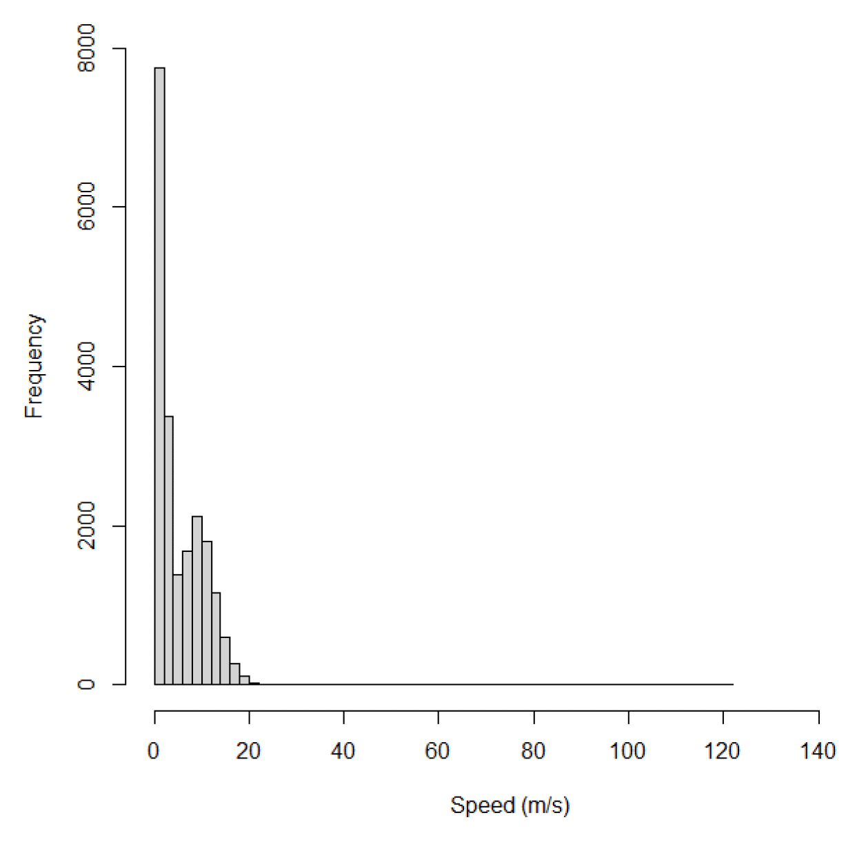
The dataset for kittiwake at Flamborough Head and Bempton Cliffs included 20,287 data points from 36 individuals on 305 foraging trips. Across all behaviours, speeds recorded for offshore movements using GPS ranged from 0.01 m/s to 127 m/s, with a median of 3.08 m/s (95% CIs 1.34 – 8.99) (Figure 24).
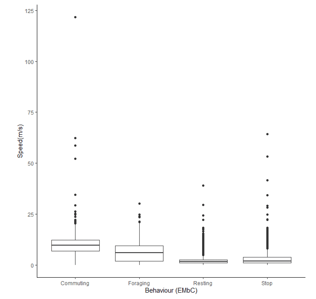
Following behavioural classification with EMbC, there were clear differences in flight speed between behaviours (Figure 24). Commuting flight speeds were faster than foraging flight speeds (Table 13) at 9.73 m/s (95% CIs 6.93 – 12.33) in comparison to 6.07 m/s (95% CIs 1.85 – 9.46). For both foraging and commuting flight, trajectory speeds derived from EMbC with reference to step length were noticeably slower than the instantaneous speeds measured using GPS.
| Colony (n birds) | Data grain | Speed type | 1 (floating) | 2 (Stop) | 3 (commuting) | 4 (forage/search) |
|---|---|---|---|---|---|---|
| Flam (36) | 300s | Instantaneous | 1.66 (1.01,2.57) | 1.84 (0.96,3.82) | 9.73 (6.93,12.33) | 6.07 (1.85,9.46) |
| Flam (36) | 300s | Trajectory | 0.54 | 0.38 | 7.58 | 3.90 |
3.2.6. Gannet Flamborough Head and Bempton Cliffs
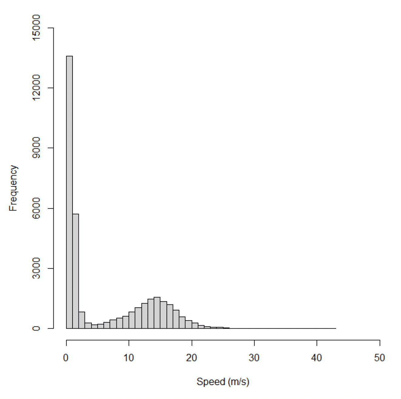
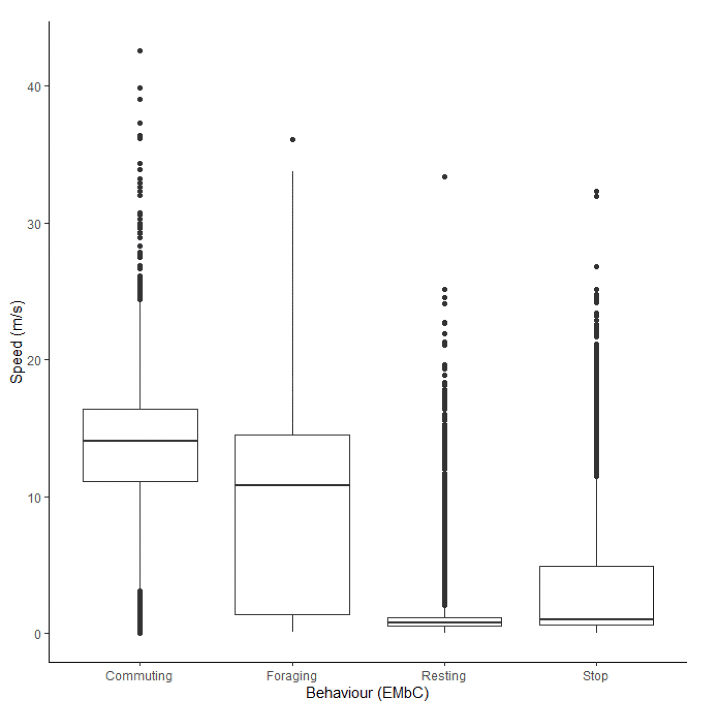
The dataset for gannets at Flamborough Head and Bempton Cliffs included 34,120 data points from 10 individuals on 301 foraging trips. Across all behaviours, speeds recorded for offshore movements using GPS ranged from 0.02 m/s to 42.60 m/s, with a median of 1.36 m/s (95% CIs 0.71 – 12.79) (Figure 26).
Following behavioural classification with EMbC, there were clear differences in flight speed between behaviours (Figure 27). Commuting flight speeds were faster than foraging flight speeds (Table 14) at 14.01 m/s (95% CIs 11.13 – 16.44) in comparison to 10.79 m/s (95% CIs 1.41 – 14.51).
| Colony (n birds) | Data grain | Speed type | 1 (floating) | 2 (Stop) | 3 (commuting) | 4 (forage/search) |
|---|---|---|---|---|---|---|
| Flam (10) | 300s | Instantaneous | 0.80 (0.55, 1.15) | 1.04 (0.60,4.96) | 14.01 (11.13,16.44) | 10.79 (1.41,14.51) |
| Flam (10) | 300s | Trajectory | 0.46 | 0.50 | 10.80 | 6.29 |
3.2.7. Flight speed summary
Across all three species, commuting flight speeds were substantially faster than foraging flight speeds (Table 15). At present, recommended generic speeds for the three species considered here are 13.1 m/s for lesser black-backed gull and kittiwake (Alerstam et al., 2007) and 14.9 m/s for gannet (Pennycuick, 1997). Regardless of the approach taken to estimate flight speed from GPS data, these generic flight speeds are substantially faster than those observed in the data presented here, with the exception of the commuting flight speed for gannet.
Comparison of trajectory and instantaneous speeds highlighted that whilst the two are strongly correlated, the trajectory speeds are slower than instantaneous speeds. More detailed analysis of the lesser black-backed gulls revealed that these correlations were strongest for commuting speeds. Whilst a higher sampling rate resulted in trajectory speeds that more closely matched the instantaneous speeds, even at the fastest rate considered here (300s), a noticeable difference remained. This highlights the importance of using instantaneous rather than trajectory speeds.
For lesser black-backed gulls, estimated speeds for each state were broadly consistent across all three sites, regardless of the method used to derive them. As might be expected, commuting flight speeds are noticeably faster than foraging flight speeds with both floating and perching speeds slower still. Generally, differences in sampling rate did not have a significant impact on the speed estimated. However, commuting speeds estimated using HMMs were a closer match to the instantaneous speeds than those estimated using EMBC. For foraging speeds, the reverse was true.
| Species | Colony | State | Trajectory | Instantaneous | |||
|---|---|---|---|---|---|---|---|
| HMM | EMBC | ||||||
| 300 | 3600 | 300 | 3600 | ||||
| Lesser Black-backed Gull | Walney | Floating | 0.32 (0.13-0.59) | 0.42 (0.27,0.60) | 0.43 (0.26,0.59) | 1.32 (0.77,2.05) | 1.30 (0.76,1.94) |
| Perching | 0.45 (0.31-0.62) | 0.26 (0.08,0.51) | 0.23 (0.08,0.50) | 1.51 (0.76,2.61) | 1.69 (0.77,2.66) | ||
| Commuting | 9.17 (7.42-11.26) | 8.15 (5.51,10.54) | 7.49 (4.19,9.97) | 9.51 (7.12,11.88) | 9.53 (6.85,11.82) | ||
| Foraging | 3.55 (1.99-5.39) | 5.25 (2.39,8.59) | 4.25 (2.06,7.11) | 7.94 (2.59,10.79) | 6.87 (1.82,10.57) | ||
| Skokholm | Floating | 0.34 (0.22-0.46) | 0.52 (0.3,1.35) | 0.54 (0.3,1.37) | 1.66 (1.14,2.41) | 1.62 (1.1,2.43) | |
| Perching | 1.49 (1.23-1.71) | 0.24 (0.14,0.39) | 0.24 (0.13,0.39) | 1.47 (0.95,2.19) | 1.45 (0.96,2.17) | ||
| Commuting | 9.43 (7.72-11.67) | 8.76 (6.28,11.06) | 8.58 (6.13,11.21) | 10.14 (7.85,12.84) | 10.05 (7.61,12.79) | ||
| Foraging | 1.49 (0.44-3.70) | 4.53 (1.99,7.92) | 4.64 (1.97,7.84) | 7.06 (1.81,10.83) | 7.03 (1.74,10.6) | ||
| Orfordness | Floating | 0.26 (0.15-0.37) | 0.74 (0.48,0.95) | 0.75 (0.51,0.93) | 0.85 (0.6,1.13) | 0.87 (0.63,1.14) | |
| Perching | 0.81 (0.64-0.99) | 0.63 (0.28,1) | 0.65 (0.25,1.05) | 0.95 (0.52,3.85) | 0.89 (0.54,4.19) | ||
| Commuting | 9.65 (7.94-11.84) | 8.59 (6.09,10.95) | 8.07 (5.08,10.57) | 9.7 (7.36,12.25) | 9.37 (7.06,12.03) | ||
| Foraging | 2.41 (1.03-4.48) | 5.67 (3.23,8.39) | 5.67 (3.12,8.92) | 7.69 (1.71,10.75) | 7.98 (2.17,10.91) | ||
| Kittiwake | Flamborough Head to Bempton Cliffs | Floating | 0.54 | 1.66 (1.01,2.57) | |||
| Stop | 0.38 | 1.84 (0.96,3.82) | |||||
| Commuting | 7.58 | 9.73 (6.93,12.33) | |||||
| Foraging | 3.9 | 6.07 (1.85,9.46) | |||||
| Gannet | Flamborough Head to Bempton Cliffs | Floating | 0.46 | 0.80 (0.55, 1.15) | |||
| Stop | 0.5 | 1.04 (0.60,4.96) | |||||
| Commuting | 10.8 | 14.01 (11.13,16.44) | |||||
| Foraging | 6.29 | 10.79 (1.41,14.51) | |||||
3.3. Flight height
3.3.1. Lesser black-backed gull
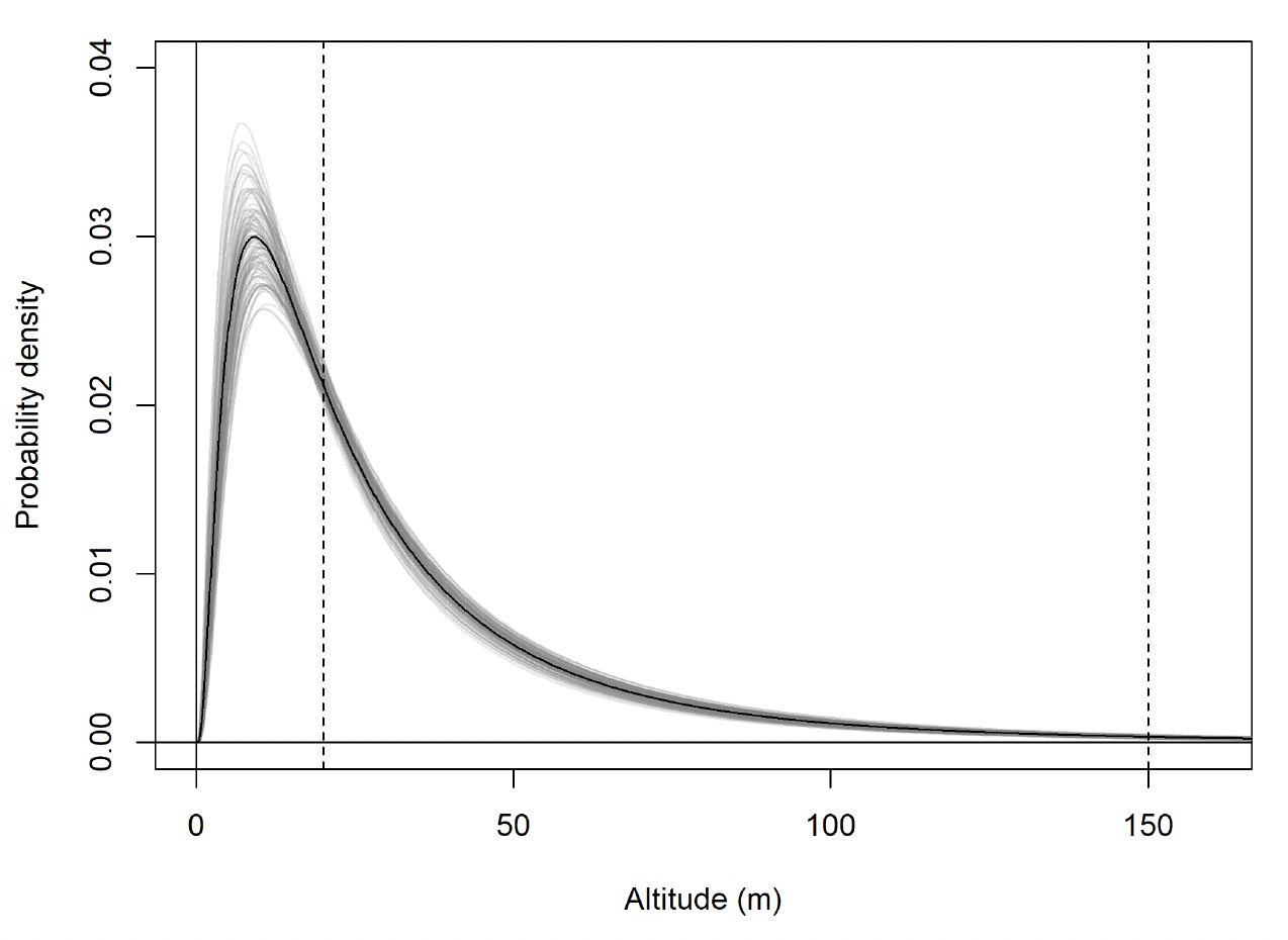
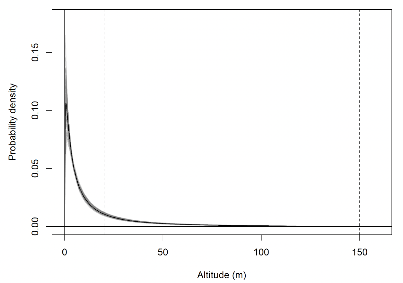
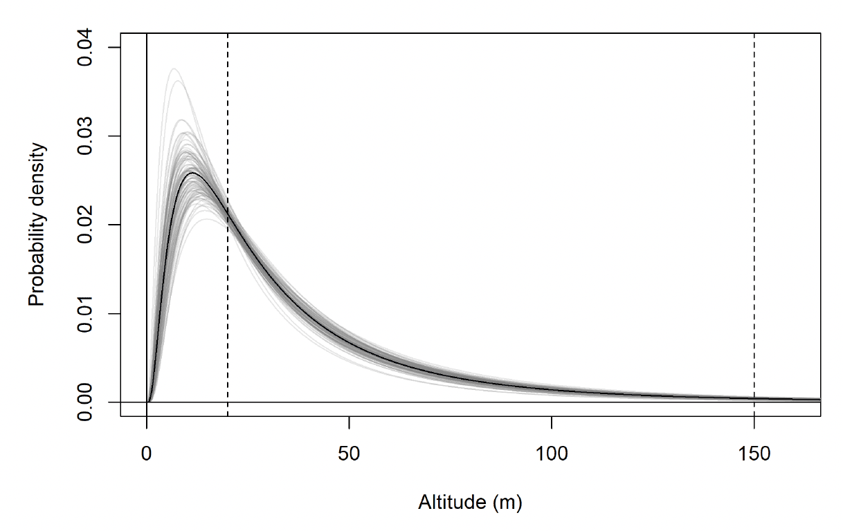
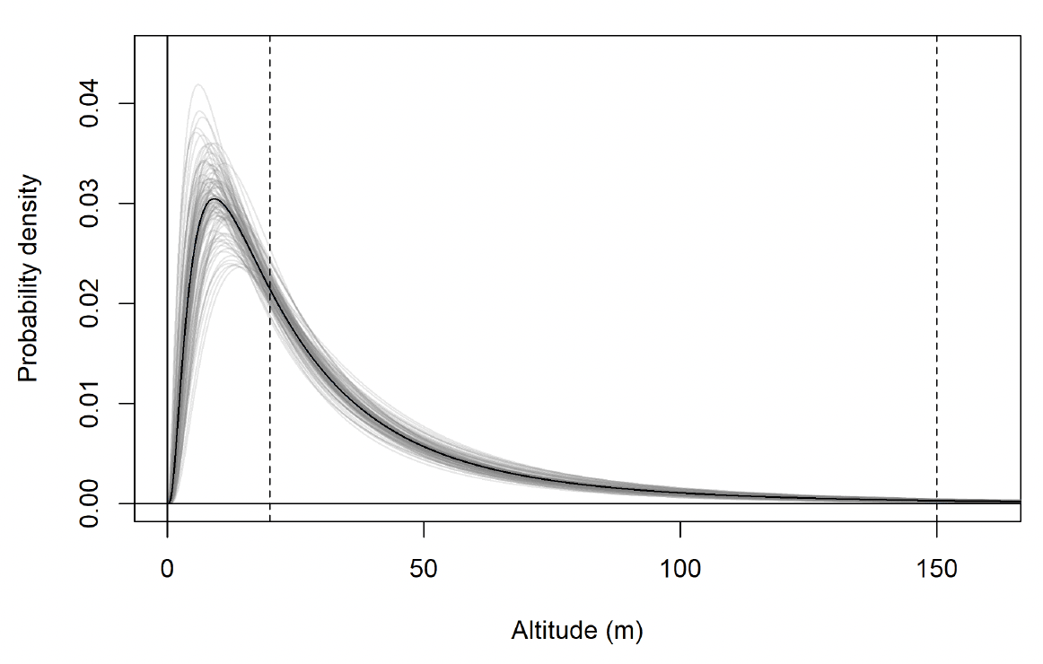
For lesser black-backed gull modelled flight height distributions, all parameters had R-hat values of <1.1 and chains had visually converged. There was correlation between the chains for mu and sd for each behavioural state or behavioural state:colony combination. There was a clear difference between modelled commuting and foraging/searching height distributions (Fig. 28). Whilst there was some overlap between these distributions, the bulk of foraging/searching flight was considerably lower than commuting flight.
The fitted flight height distributions were generally similar in shape between behaviours. The distribution for foraging flight was characterized by a low estimated mean, resulting in a peak in probability density close to zero metres. For commuting flight, the peak was at 9.2m.
a)
b)
3.3.1.1. Inter-colony similarities
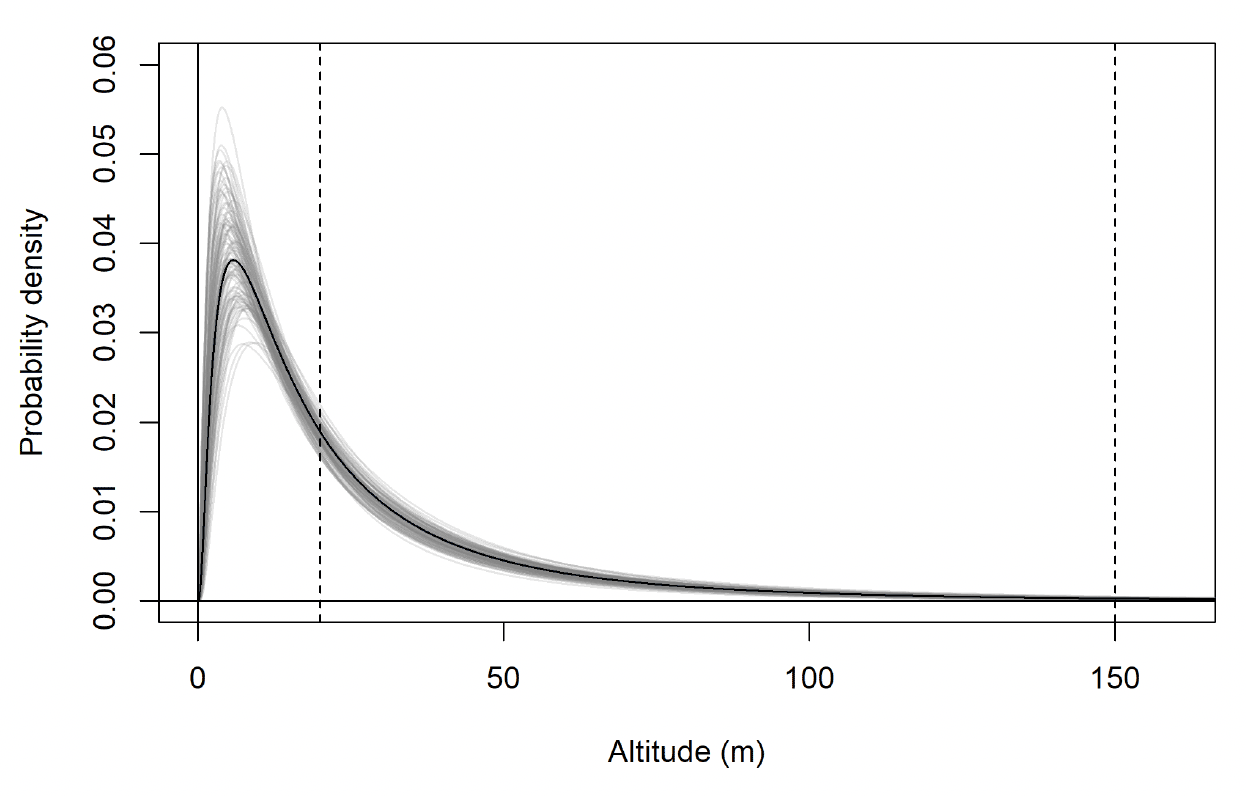
The modelled flight height distributions for lesser black-backed gull commuting height differed little between colonies (Figures 29 and 30; Table 16). Distributions had similar central tendency and overall shape. Individuals tagged at Orfordness typically had the lowest commuting flights, while individuals tagged at Skokholm had the highest.
Likewise, the modelled flight height distributions for lesser black-backed gull foraging/searching height differed little in central tendency or shape between colonies (Figure 30; Table 16). However, the relative order of the foraging/searching flight height distributions for different colonies was different to that for commuting height: for foraging/searching flight, individuals tagged at Walney typically had the lowest flights, while individuals tagged at Orfordness typically had the highest. However, the foraging/searching flight height distribution for Orfordness was slightly narrower: the upper limit of the 95% credible interval was 13m and 35m lower than those for Walney and Skokholm, respectively.
The proportion of flight time at risk height followed the same patterns as for the modelled flight height distributions: they were generally similar among colonies (Table 17). For commuting flight, individuals tagged at Orfordness had the lowest proportion of flight time at risk height, while individuals from Skokholm had the highest. For foraging/searching flight, individuals tagged at Walney had the lowest proportion of flight time at risk height, while individuals from Orfordness had the lowest. For individuals tagged at Walney and Skokholm, the proportion of flight time at risk height was much greater for commuting flight than for foraging/searching flight; for individuals tagged at Orfordness the same pattern was evident, but the 95% credible interval for proportion of flight time at risk height overlapped between the behavioural states.
a)
b)
c)
a)
b)
c)
| Colony | Median flight height (m) (& 95% CI) | |
|---|---|---|
| Commuting flight | Foraging/searching | |
| Orfordness | 17.5 (0.4-99.0) | 10.4 (0.0-89.7) |
| Skokholm | 25.9 (1.1-114.9) | 7.8 (0.0-124.7) |
| Walney | 21.7 (1.0-102.5) | 7.3 (0.0-102.7) |
| Colony | Projected % in 20-150m risk envelope (& 95% CI) | |
|---|---|---|
| Commuting flight | Foraging/searching | |
| Orfordness | 42.5 (34.0-50.3) | 28.5 (20.1-37.6) |
| Skokholm | 58.4 (49.9-65.8) | 24.8 (20.4-28.1) |
| Walney | 51.7 (42.6-61.7) | 23.1 (17.8-30.2) |
3.3.2. Kittiwake
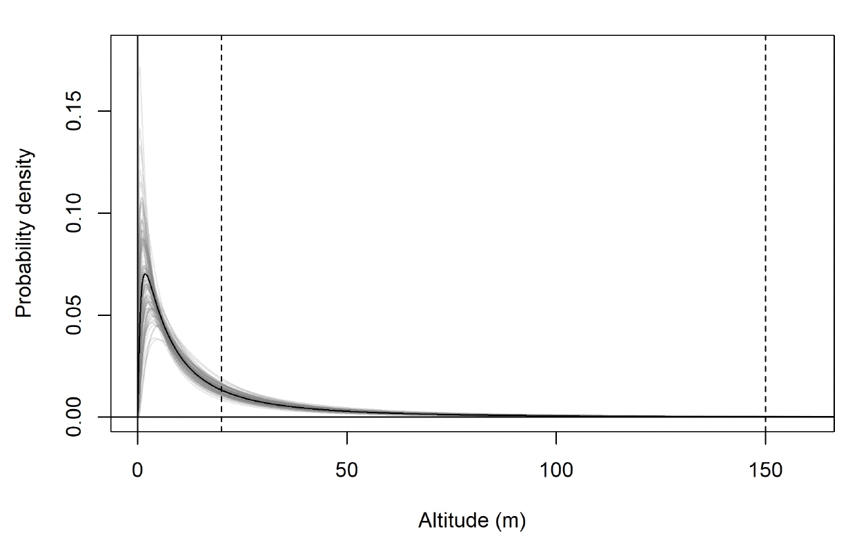
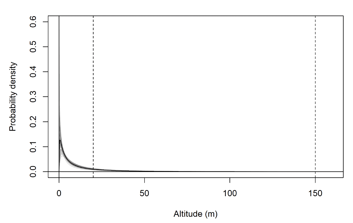
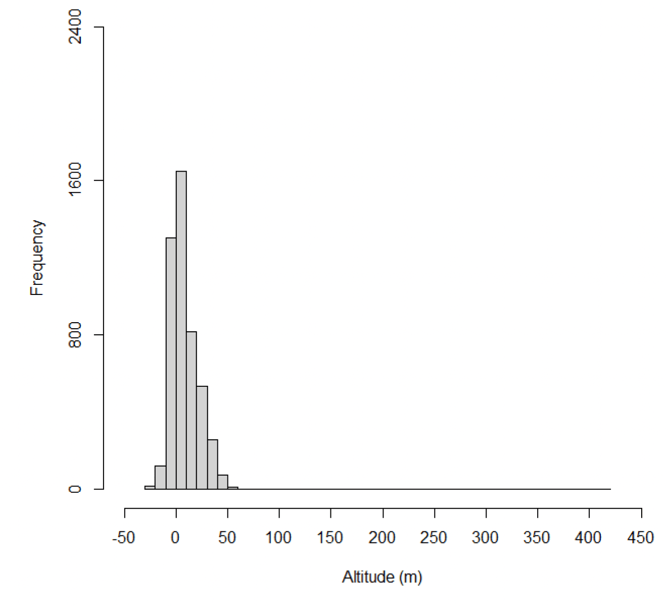
Estimates of kittiwake flight heights were obtained using altimeters from 16 individuals on 117 foraging trips. In total, 4,790 data points were obtained. Analyses of these data are ongoing (Wischnewski, Sansom, et al., in prep.), consequently a small number of negative altitudes remain in the dataset, and it is important these data are included in any analyses of flight height to ensure all errors are accounted for in final modelled distributions (Péron et al., 2020). The maximum estimated flight height was 412 m above sea level, though most data were much closer to the sea surface with a median height estimate of 4.49 m above sea level (95% CIs 0 – 1.24), and 18% of flight activity within a theoretical 20-150m collision risk window (Wischnewski, Sansom, et al., in prep).
Estimated flight heights during commuting were higher than those estimated during foraging (Figure 32, Table 18). Reflecting this, the proportion of flight activity at collision risk height during commuting flight was more than double that of the proportion at collision risk height during foraging activity (Table 19). Whilst the overall patterns in these data are likely to reflect the true patterns in flight heights (e.g., commuting birds fly higher than foraging birds), the reported values should be treated with caution as the error surrounding these estimates has not been properly quantified and accounted for in the modelling process, resulting in the negative estimates in flight height (Figures 31 & 32).
| Colony | Median flight height (m) (& 95% CI) | |
|---|---|---|
| Commuting flight | Foraging/searching | |
| Flamborough Head and Bempton Cliffs | 12.49 (4.84, 23.90) | 7.44 (0.18,19.40) |
| Colony | Projected % in 20-150m risk envelope | |
|---|---|---|
| Commuting flight | Foraging/searching | |
| Flamborough Head and Bempton Cliffs | 31 | 24 |
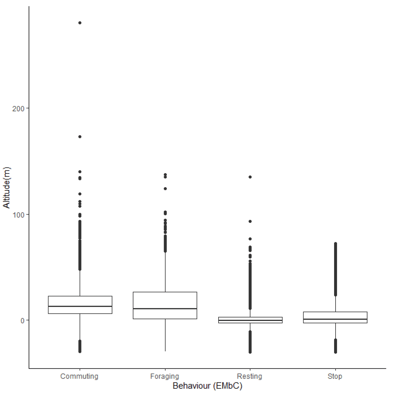
3.3.3. Gannet
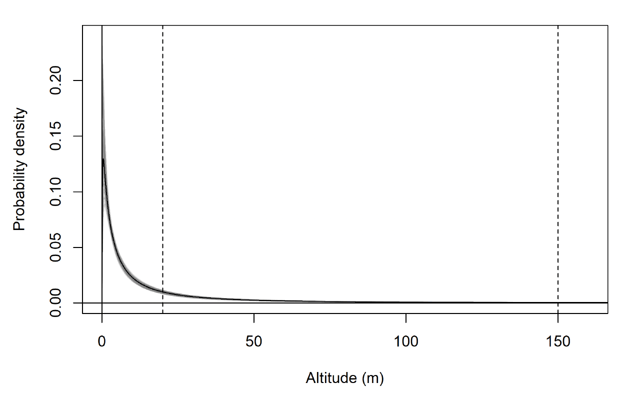
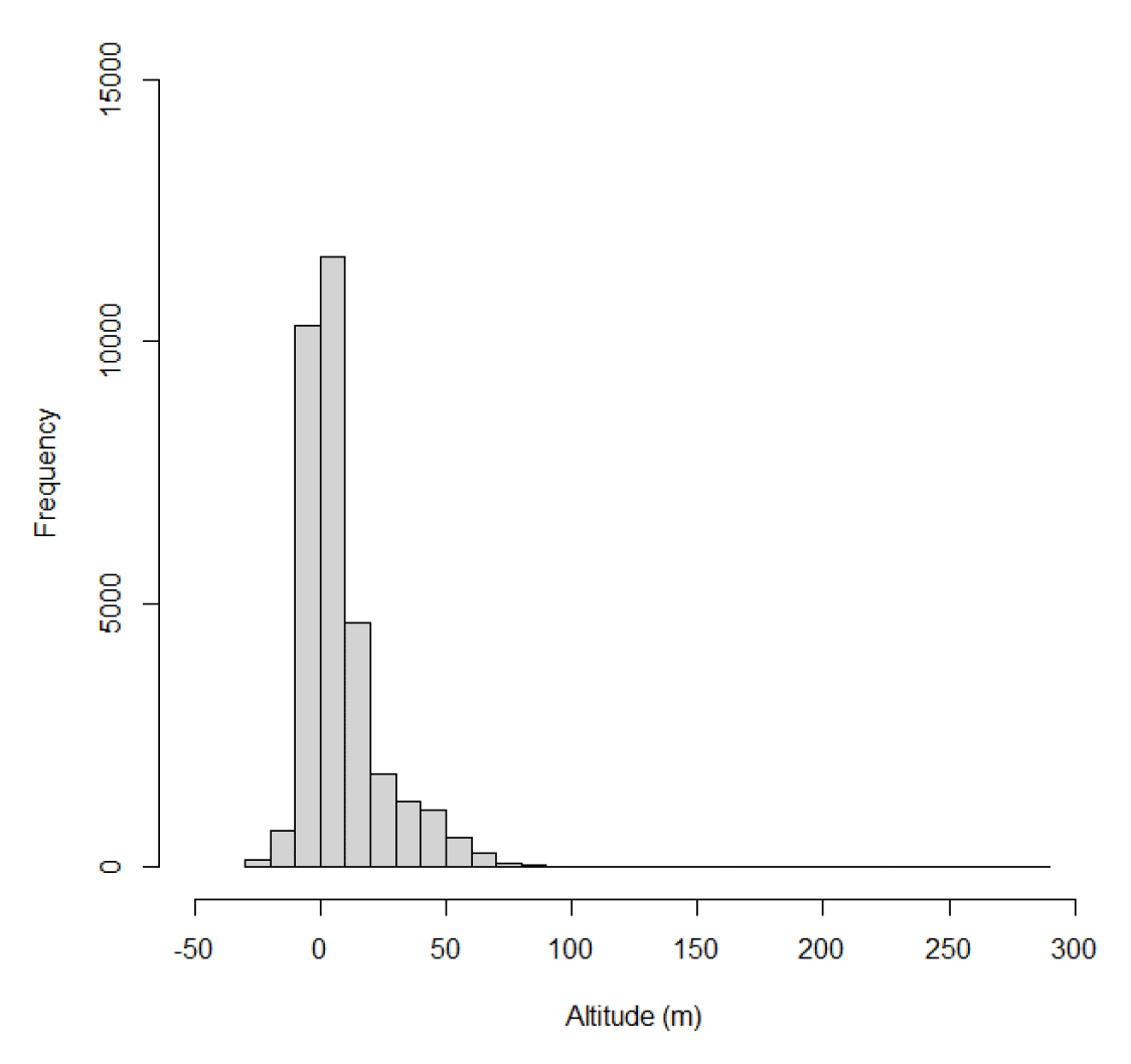
Estimates of gannet flight heights were obtained using altimeters from 10 individuals on 278 foraging trips. In total, 32,484 data points were obtained. Analyses of these data are ongoing (Wischnewski, Sansom, et al., in prep.), consequently a small number of negative altitudes remain in the dataset, and it is important these data are included in any analyses of flight height to ensure all errors are accounted for in final modelled distributions (Péron et al., 2020). The maximum estimated flight height was 280 m above sea level, though most data were much closer to the sea surface with a median height estimate of 2.76 m above sea level (95% CIs 0 – 12.63), and 15% of flight activity within a theoretical 20-150m collision risk window (Wischnewski, Sansom, et al., in prep). The inclusion of negative flight heights in the data is likely to lead to an under-estimate of the median flight height. However, in this context, the primary interest is in the proportion of birds at collision risk height. As negative flight height records are likely to relate to birds flying below a turbine rotor sweep (Péron et al., 2020), excluding these data may result in an over-estimate of the proportion of birds at collision risk height.
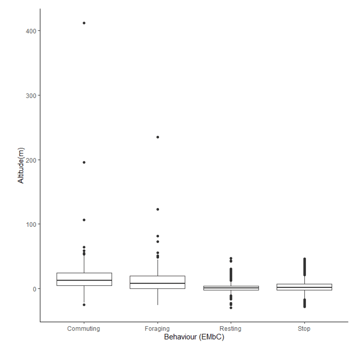
Estimated median flight heights during commuting were slightly higher than those estimated during foraging (Figure 34, Table 20). However, there was greater variability in foraging flight height than was the case for commuting flight, meaning that a slightly higher proportion of foraging flight took place at collision risk height (Table 21). Whilst the overall patterns in these data are likely to reflect the true patterns in flight heights (e.g., commuting birds fly higher than foraging birds), the reported values should be treated with caution as the error surrounding these estimates has not been properly quantified and accounted for in the modelling process, resulting in the negative estimates in flight height (Figures 33 & 34).
| Colony | Median flight height (m) (& 95% CI) | |
|---|---|---|
| Commuting flight | Foraging/searching | |
| Flamborough Head and Bempton Cliffs | 12.8 (5.97,22.77) | 10.78 (1.07,26.57) |
| Colony | Projected % in 20-150m risk envelope | |
|---|---|---|
| Commuting flight | Foraging/searching | |
| Flamborough Head and Bempton Cliffs | 29 | 32 |
3.3.4. Flight Height Summary
For lesser black-backed gull and kittiwake, there were clear differences in the median flight heights estimated for commuting and foraging flight (Table 22). For gannet, there appeared to be greater overlap in foraging and commuting flight heights. Consistent with previous studies (A. Johnston et al., 2014), lesser black-backed gulls had higher flight heights than either gannet or kittiwake. Reflecting this, lesser black-backed gulls also spent a greater proportion of time within our projected 20-150m collision risk envelope than was the case for the other species (Table 23). Commuting flight heights were similar for gannet and kittiwake (Table 22). However, during foraging flight, gannets tended to fly higher than kittiwakes, spending a greater proportion of time at collision risk height.
| Species | Median flight height (m) (& 95% CI of flight height) | |
|---|---|---|
| Commuting flight | Foraging/searching | |
| Lesser black-backed gull | 22.1 (1.0-107.2) | 8.2 (0.0-107.2) |
| Kittiwake | 12.5 (4.8,23.9) | 7.44 (0.18,19.40) |
| Gannet | 12.8 (5.9, 22.7) | 10.78 (1.07,26.57) |
| Species | Projected % in 20-150m risk envelope (& 95% CI) | |
|---|---|---|
| Commuting flight | Foraging/searching | |
| Lesser black-backed gull | 52.1 (45.8-57.6) | 25.2 (21.7-29.5) |
| Kittiwake | 31 | 24 |
| Gannet | 29 | 32 |
Contact
Email: ScotMER@gov.scot