Understanding seabird behaviour at sea part 2: improved estimates of collision risk model parameters
Report detailing research using GPS tags to track Scottish seabirds at sea.
2. Methods
2.1. Data sets
Building on the analyses carried out in Thaxter et al. (2019), we estimate nocturnal activity, defined as the period from sunrise to sunset as per Band (2000) and Forsythe et al. (1995), from GPS tagging data, and estimate behaviour-specific flight heights and flight speeds. In addition to the data considered in Thaxter et al. (2019), data were also available for 36 kittiwakes and 10 gannets fitted with University of Amsterdam (UvA) GPS tags by RSPB within the Flamborough Head and Bempton Cliffs SPA. Analysis of nocturnal activity levels considered data collected using both IGotU GT-120 (Mobile Action Technology, Taipei, Taiwan) and UvA GPS tags (Table 1).
Given the data recording capabilities of the different tags, analyses of flight height and flight speed were restricted to the UvA tags (Table 1). For lesser black-backed gulls, analyses of flight heights were based on GPS estimates, for gannets and kittiwakes flight height estimates were based on altimeter data analysed by RSPB as part of ongoing work (Babcock et al., 2018). A summary of the data sets and analyses considered in this report is presented in Table 1.
| Species | Colony | Tag | Sample Size | Nocturnal Activity | Flight Speed | Flight Height |
|---|---|---|---|---|---|---|
| Kittiwake | Isle of May | IGotU | 50 | √ | ||
| Orkney | IGotU | 86 | √ | |||
| Colonsay | IGotU | 84 | √ | |||
| Bempton Cliffs | IGotU | 104 | √ | |||
| Bempton Cliffs | UvA | 16 | √ | √ * | √ ** | |
| Lesser Black-backed Gull | Walney | UvA | 37 | √ | √ | √ |
| Orfordness | UvA | 24 | √ | √ | √ | |
| Skokholm | UvA | 24 | √ | √ | √ | |
| Gannet | Bass Rock | IGotU | 133 | √ | ||
| Alderney | IGotU | 61 | √ | |||
| Bempton Cliffs | UvA | 10 | √ | √ * | √ ** |
*Analyses undertaken by RSPB as part of ongoing work prior to award of contract;
**Analysis of altimeter data undertaken by RSPB as part of ongoing work.
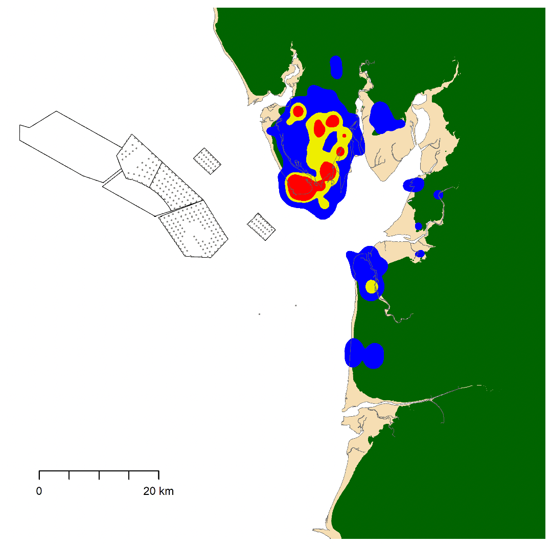
Initially, we hoped to carry out similar analyses for herring gulls. However, examination of available GPS tracking data for this species suggested that, due to movements largely being restricted to onshore areas, there were insufficient data for analysis of offshore behaviour (e.g., Figure 1).
2.2. Behavioural classification
Previous analyses were based on Hidden Markov Models (HMMs) (Thaxter et al., 2019). A Hidden Markov Model (HMM) is a state-space continuous time movement approach that includes a ‘hidden’ component modelled as a Markov process, that allows states to be estimated informed by the relationships to an ‘observed component’ of the model (in this case, based on the step length between GPS fixes and turning angle). As a pre-requisite, this analysis required that time steps between consecutive GPS fixes were at a constant ‘regularised’ sampling rate, such that time steps were precisely the same for all points. Data were regularised to a constant spatial and temporal spacing using R packages ‘crawl’ (Johnson et al., 2008) and ‘momentuHMM’ (McClintock & Michelot, 2018). The ‘crawl’ model was used to fit a correlated random walk-through locations (Johnson et al., 2008), and further allowed interpolative prediction of points at five-minute intervals. Initial analyses suggested that this approach posed particular problems for the analysis of nocturnal activity.
The HMM analyses (Thaxter et al., 2019) classified points as floating, foraging or commuting behaviour, with an additional perching classification for lesser black-backed gull. In assessing activity levels, it is necessary to consider the proportion of time spent foraging and commuting in relation to the proportion of time spent perching or floating. However, these classifications are based on data collected away from the breeding colonies. Consequently, it is necessary to account for time spent at the colony in addition to time spent in perching or floating behaviour when classifying birds as not active. However, for a number of reasons, there may be biases associated with GPS points recorded when birds are at their colony. These include the use of GPS fences to preserve battery life by recording data at a lower temporal resolution when birds are at their breeding colonies, and the potential for the surrounding habitat (e.g., cliffs) to impair the ability of GPS tags to communicate with satellites and/or, in the case of the UvA tags, for solar panels to receive sufficient light to recharge tag batteries. Regardless of the cause, if birds spend more time at the colonies at night than during the day, as seems likely, these biases are likely to produce an over-estimate of nocturnal activity levels. The need for regularised time steps in HMMs means that adding time spent at colonies back into the data, in order to overcome these biases, is not straightforward.
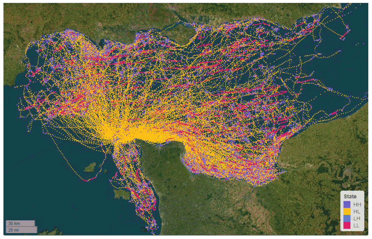
A second approach was also used to identify the same four-level behavioural states described above for the HMM. Expectation-Maximisation Binary Clustering (EMbC) is a further state-space approach that uses a Gaussian mixture model (see Garriga et al., 2016 for more details). Unlike the HMM, the EMbC approach does not strictly need a regularised interpolated dataset, as it is based on GPS speed and turning angle, rather than distance within a constant time period. The EMbC model by default allows classification of four states grouped by: low speed, low turn (‘LL’, = floating); low speed, high turn (‘LH’ = stopped); high speed, low turn (‘HL’ = commuting); and high speed, high turn (‘HH’ = potential foraging/searching) (Figure 2). Whilst the definitions of most of these categories are fairly clear, the LH category is less obvious. The low speed indicates that birds are not altering their locations, while the high turning angle indicates birds are altering their orientation regularly, implying that they are active. This category is likely to reflect a combination of maintenance behaviour and foraging from the sea surface. For simplicity, in this report the behaviour is referred to as “stopped” however, it is important to acknowledge that it may also include aspects of foraging behaviour.
By using the expectation maximisation algorithm, the EMbC approach seeks the most optimised split in the data but does not require prior information for perceived delineations for each category as with HMMs above. The EMbC approach can handle temporal data "gaps" in the dataset. However, it is generally best applied on a reasonably regular dataset, i.e., without excessively variable sampling resolutions, and so the data were filtered to a rate of five minutes, for a comparable assessment to the HMMs above. The resulting classifications of foraging and commuting behaviour were broadly consistent with those obtained from HMM.
2.3. Nocturnal activity
We follow the approach of (Furness et al., 2018) in assigning the timing of GPS points to dawn, daylight, dusk and night using the ‘sunriset’ and ‘crepuscule’ functions in the R package “maptools” (Bivand & Lewin-Koh, 2021). We then analyse activity levels using a Generalized Linear Mixed Model (GLMM) with a binomial error distribution and a logit-link. Using this approach, we analyse the proportion of time active (behavioural states HL and HH) in relation to the light level classifications above. For each species and colony combination, we fitted a model for each year in which data were collected. For our models, we include light levels (dawn, day, dusk, night) as a categorical fixed effect and, bird identification as a random effect. The model was parameterised as follows:
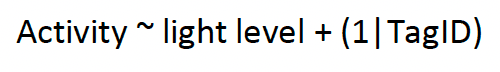
[1]
The outputs from these models are used to quantify the proportion of time birds are active in relation to each light level. For the purposes of collision risk modelling, nocturnal activity levels are the proportion of time birds are active at night relative to their activity during the day. Consequently, to estimate nocturnal activity levels for use in collision risk models, we divided the proportion of time active at night by the proportion of time active during the day. We then compared nocturnal activity levels between species, sites, and colonies.
2.4. Flight speed
2.4.1. Instantaneous speed estimates for foraging and commuting flight
In Thaxter et al. (2019), estimates of flight speed were obtained for foraging and commuting flight based on the straight line distance travelled between sampling intervals. However, concern was raised that the temporal resolution of the fixes meant that estimates based on this approach may under-estimate true speed if birds were not travelling in a straight line at the time. However, UvA tags also collect vector-based instantaneous speed measures, taken over a short period for each GPS fix, resulting in x, y, and z speeds in m/s. These can be combined into a “3D” vector-based instantaneous speed for each GPS fix (i) through the following equation:

[2]
Using the EMbC classifications of behaviour, these speeds were then summarised for points classified as foraging and commuting flight for lesser black-backed gull, gannet and kittiwake.
2.4.2. Comparison of instantaneous and trajectory speed
The EMbC model was assessed for each species at a 300 s rate (t), reflecting the overall “base” rate of GPS sampling protocols for each project (Table 1). A trajectory speed was also estimated, based on the distance travelled (d) between sampling intervals, measured as:
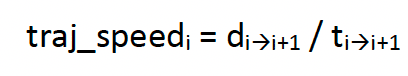
[3]
For the lesser black-backed gull data from Walney, Skokholm and Orfordness, instantaneous and trajectory speeds were considered in more detail. The subsampling regime removed often faster rates (up to 5s) that had been collected for finer-scale investigations into movements within wind farms. Thus, although trajectory speeds were sometimes available for these “bursts” of activity, the ones used for comparison to instantaneous speeds were the sub-sampled re-calculated ones at the base rates described above, enabling a fairer comparison across the rest of the dataset.
Point estimates of bird flight speeds are likely to be correlated with the immediately preceding estimates. These correlations can introduce bias into any subsequent analysis that influence the resulting parameter estimates. To avoid unduly biasing parameter estimates, an initial investigation was made into the autocorrelation within the data for both instantaneous and trajectory speed parameters. These assessments were carried out at the individual bird level through Auto-Correlation Function (ACF) plots, examining the ACF for the five-minute rate used in the EMbC, and subsequent data degradation to coarser rates of 600s, 900s, 1200s, 1800s and 3600s, with the ACF re-examined for each sub-sampling rate level, and examined for each bird in each breeding season year.
We then used both simple linear regression to compare the pairwise point-level data for each speed type, and further fitted a Generalized Linear Mixed Effects Model to compare differences in the relationships between speed types over behavioural states; a model was therefore specified as:

[4]
Given the focus of the work, a further model investigating just offshore was therefore considered further for behavioural states, simplifying the above model to remove the offshore three-way interaction, for which results are presented:

[5]
where speed_type is a factor of instantaneous or trajectory, offshore a factor of onshore or offshore, and random effects if TagID nested within year were specified and the error distribution (ɛ) being a log-transformed gaussian distribution (which gave superior residuals and quickest model run time). This model was specified using R package glmmTMB (Brooks et al., 2017) and further tests of autocorrelation were carried out with R package DHARMa (Hartig, 2022). The slope and significance of the relationship was then examined for each interaction for all factor levels of state. Estimates from the above model were examined using estimated marginal means (R package emmeans, Lenth, 2022).
For each EMbC state (1-4), we further visualised the two types of speed measures. The approach for comparison was one of a distribution comparison and summary of basic statistics of error around the measures, being histograms, and non-parametric boxplot statistics.
2.5. Flight Heights
2.5.1. Bias in GPS altitudes
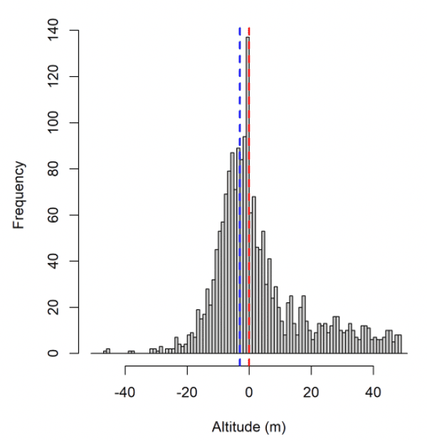
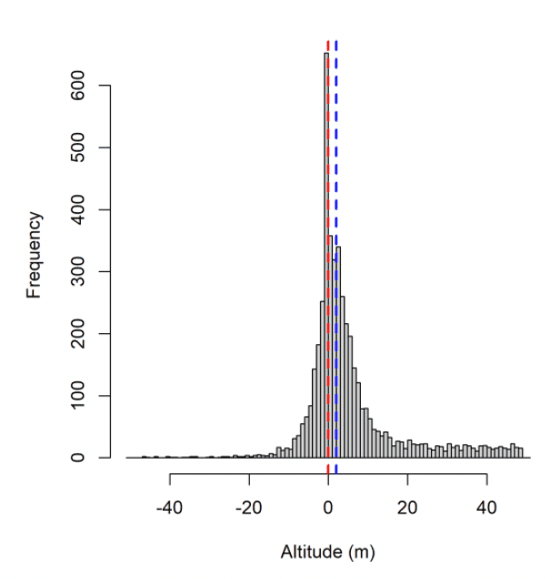
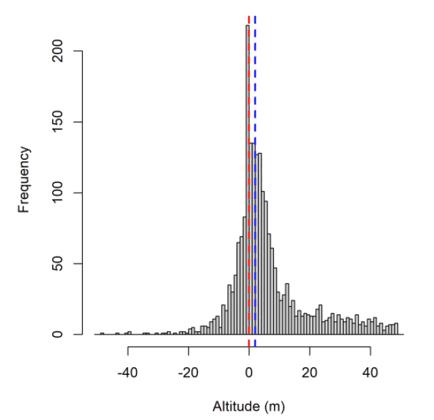
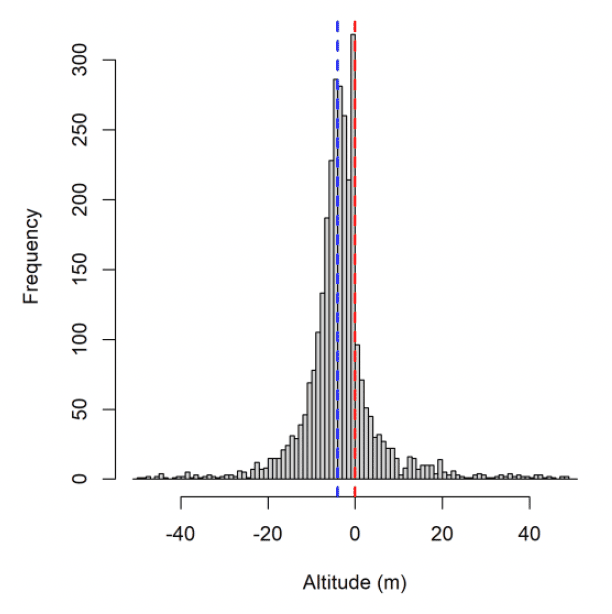
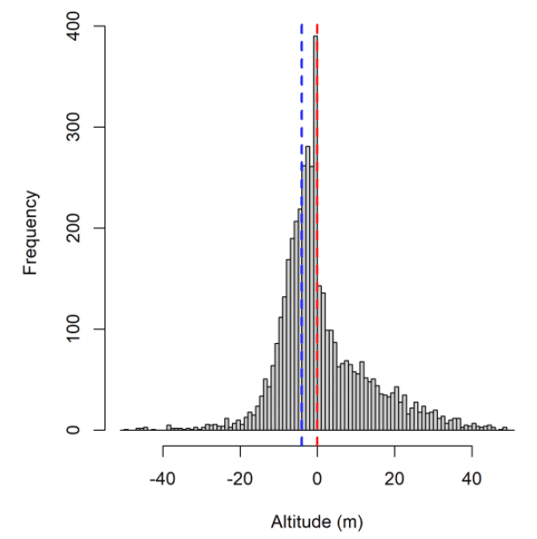
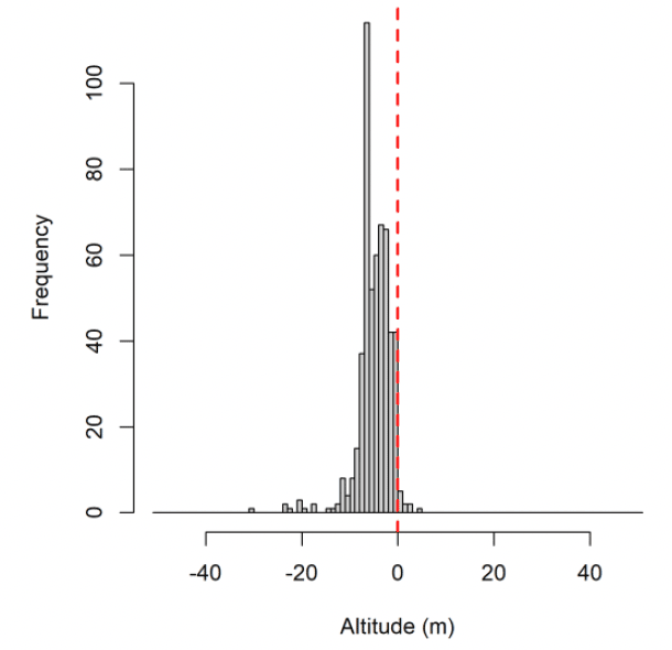
For lesser black-backed gull at Orfordness (but not Skokholm or Walney), and gannet and kittiwake at Flamborough Head and Bempton Cliffs, the bulk of the distribution of raw GPS altitudes was negative (Fig. 3). This suggests that the GPS altitude measurements are negatively biased in the southern North Sea. An ecological cause for this bias was explored: that birds are preferentially going out at low tide. If this was a cause of the altitude bias, it was not the sole cause: lesser black-backed gull altitude while stopped on land was also biased below the Digital Elevation Model (DEM) for birds tagged at Orfordness (not shown), and the bulk of GPS altitudes from a test tag left at the shoreline at Orfordness in 2011 were negative (Fig. 3f).
It could instead be that there was error in the calculation of altitude over mean sea level from altitude over the ellipsoid: perhaps due to spatially variable error in the geoid. There was some evidence that the altitude bias varied smoothly across the study areas, suggesting there are issues with the model of mean sea level used. Furthermore, a recent test tag at Havergate (near Orfordness) had no altitude bias. However, the error in the height of true mean sea level relative to the geoid is almost entirely less than 1m, considerably less than the average bias in our dataset. Whilst the bulk of the GPS altitude distribution is below zero, the modal GPS altitude for kittiwake and gannet is zero. Consequently, the cause of the altitude bias is unclear.
We applied a correction to account for this based on the median altitude estimate of birds classified as floating on the sea surface. Assuming that instances of floating behaviour are distributed evenly across the tidal cycle, the median estimated flight height should reflect sea-level, and this value can be subtracted from GPS estimated flight heights to correct for biases in these estimates. This will only be an informal solution to the problem, for two reasons. Firstly, the altitude bias varied smoothly within the study areas: so, the median altitude of birds floating on water is only a useful estimate of altitude bias on average at a colony, and any uncertainty in the average bias is not propagated into the remainder of the analysis. Secondly, although the bulk of the GPS altitudes for kittiwake, gannet and Orfordness lesser black-backed gulls are below zero, an unknown process in the data-generating process results in the modal GPS altitude for kittiwake and gannet being zero; after adjustment this is above zero. If the zero-metre mode of the GPS altitudes has an ecological cause (rather than being caused by observation processes), then this aspect of the distribution is distorted by our adjustment.
Where a high proportion of GPS altitudes are negatively biased, this may influence flight height distributions because the lognormal distribution used to model imperfectly observed true flight heights only has support over the set of positive numbers. Any negative flight height observations will be classified as measurement errors by the model and may lead to estimates of very small positive true altitudes (highly negative values on the log scale). Even after corrections based on measurements of birds classified as floating on the sea surface, a high proportion of altitude measurements for kittiwake and gannet remained below zero. Consequently, GPS measurements of flight heights from gannet and kittiwake were not considered as part of further analyses.
a)
b)
c)
d)
e)
f)
2.5.2. Lesser black-backed gull
GPS altitude measurements are subject to error arising from various processes (Péron et al. 2020). The hierarchical model framework, separating observation error from process error, is ideal for properly accounting for GPS error when estimating species’ flight height distributions. Here we adapt a hierarchical model developed by Ross-Smith et al. (2016) to estimate the flight height distributions of lesser black-backed gulls.
Analyses were restricted to GPS points classified by EMbC as commuting or foraging. Points with uncertain classification (probability < 0.9) were excluded from analysis. To account for autocorrelation, and following Ross-Smith et al. (2016), data were sub-sampled to one point every 60 minutes. To focus solely on flight height over sea, onshore fixes were removed. After cleaning this left a dataset of 10,461 altitude measurements for lesser black-backed gulls.
The model structure we use for our two research questions is simpler than that of Ross-Smith et al. (2016), in that we do not discretize flight height by ‘location’ (terrestrial/coastal/marine) or by light-level. For the first research question, we discretize flight height by behaviour; for the second we discretize flight height by behaviour and colony. To help separate observation error from process error, we used the number of satellites associated with each flight height measurement (specifically, the number of satellites used for a given fix subtracted from 14, the maximum number of satellites used for any fix) as a covariate of observation error.
We assume that the observed altitude data obs are drawn from a normal distribution with mean alt and variance y2. alt represents the true unobserved altitude, and y is the sum of an intercept δ and a linear effect (slope θ) of the number of satellites nsat (see above). For observation i,
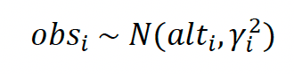
[6]
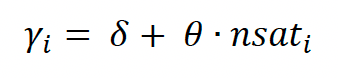
[7]
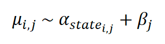
On the log scale, we assume that the logarithm of the latent true altitude alt is drawn from a normal distribution with mean μ and variance σ2. μ is the sum of an intercept α and an individual random effect ß. In the first models α and σ are estimated separately for each behavioural state. In the second model α and σ are estimated separately for each behavioural state and by colony. For observation i and individual j (structure of first model only),
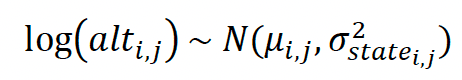
[8]
[9]
Model parameters were estimated in a Bayesian framework using Markov Chain Monte Carlo (MCMC) sampling for inference and with vague priors. Parameter estimation was implemented in “Just Another Gibbs Sampler” (JAGS) (Plummer 2003), accessed using the runjags package (Denwood 2016) in R (R Core Team 2020). To minimize autocorrelation in the chains only one in every 10 iterations was retained. The first 30,000 iterations were discarded as burn-in, and the following 200,000 iterations were used for estimating the posterior probability distributions of the parameters.
Model convergence was assessed by visual inspection of MCMC trace plots and the Gelman-Rubin statistic R-hat. Models were considered to have converged on the posterior probability distribution if the MCMC chain plots were well-mixed and if R-hat was less than 1.1, for all parameters. Correlation between the MCMC traces was also examined to give indications of interdependencies among parameters.
2.5.3. Kittiwake and Gannet
As the GPS estimates of flight height for kittiwake and gannet were not considered reliable for the purposes of these analyses, we considered estimates that were collected using altimeters deployed concurrently with the GPS tags. These data were collected and analysed by RSPB as part of ongoing work (Wischnewski, McCluskie, et al., in prep.; Wischnewski, Sansom, et al., in prep.).
Atmospheric pressure declines with altitude and, consequently, the pressure measurements recorded using altimeters can be used as a proxy for the flight altitude of birds. This requires a baseline estimate of local atmospheric pressure at a known altitude. This can be compared to the pressure recorded by the altimeter which is then converted into an estimate of flight altitude using established relationships between air pressure and altitude. For the purposes of this study, estimates of air pressure were obtained from a local weather station in Bridlington, close to the study site.
The data considered in these analyses were collected from 10 gannets and 16 kittiwakes. As above, GPS data collected alongside the altimeter data were used to partition points into resting, stopped, foraging, and commuting behaviour using EMbC with sampling intervals of 5 minutes. The altimeter estimates of flight altitude for foraging and commuting birds were then compared. In contrast to the flight heights estimated using GPS, the observation error process for altimeter flight height estimates has not been modelled as this is part of ongoing work. Consequently, a small proportion of flight height estimates for both species are below sea level.
Contact
Email: ScotMER@gov.scot