Scottish Marine and Freshwater Science Vol 6 No 12: The demography of a phenotypically mixed Atlantic salmon (Salmo salar) population as discerned for an eastern Scottish river

Supplements

Supplement A

Definition of the Grilse Error Correction Procedure used in this paper.

The mis-reporting of 1 SW (or grilse) salmon as multi-sea-winter fish was first documented by Shearer (1992), who noted that angler's distinctions were often carried out on the basis of fish weight without reference to scale samples. Bacon et al. (2010) give a statistically sound methodology for such distinction on a probabilistic basis, but that methodology was not available at the time the historical data used in this study was compiled. Moreover, the individual size and date of capture information which would facilitate retrospective application of the technique were not required parts of the reporting, and are thus not present in the data available to us.

MacLean, Smith and Laughton (1996) carried out a case-study of two Speyside estates, where scale samples were obtained from partial sub-samples of rod-catches, along with estimates of the overall ratio of grilse/ MSW fish from both scale-reading and angler's reports. Both (Shearer 1992) and MacLean ( FFL Pitlochry - pers.com.) state that anglers discriminations are made on the basis of simple, date-dependent, weight-thresholds, which are believed to vary between rivers, estates and even individual ghillies. Reporting done on this basis will grossly over-estimate rod-catches of MSW fish in every month in which grilse might be caught in significant numbers, especially from June onwards (Figure A.1). Table A.1 shows the weight thresholds used by the two estates in the Spey study (MacLean et al. 1996), together with the SALWRD size boundary, published by Bacon et al. (2010), for 50% of the fish being MSW.

Figure A.1 The weight-split-thresholds of the two Speyside Estates' and SALWRD discrimination boundary (see Table A.1) plotted against month of the year.

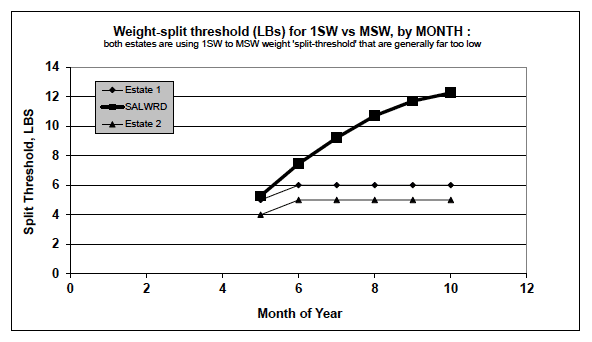
Table A.1 For each Speyside estate (Maclean et al. 1996) in each reported month the weight-threshold (in LBs) that the estate used to designate 1 SW (below) or MSW (above) salmon is given, followed by the SALWRD probabilities (Bacon et al. 2010) that such a fish would actually be 1 SW, 2 SW or 3 SW. After May, the probabilities that fish 'at the threshold' could be 2 SW or older are extremely small.

Estate	Month	Estates'weight-split threshold	SALWRD Sea Age probability
		LBs	p1 SW	p2 SW	p3 SW
1	May	5	0.64	0.36	0.00
1	Jun	6	0.91	0.09	0.00
1	Jul	6	0.99	0.01	0.00
1	Aug	6	1.00	0.00	0.00
1	Sep	6	1.00	0.00	0.00
1	Oct	6	1.00	0.00	0.00
2	May	4	0.95	0.05	0.00
2	Jun	5	0.99	0.01	0.00
2	Jul	5	1.00	0.00	0.00
2	Aug	5	1.00	0.00	0.00
2	Sep	5	1.00	0.00	0.00
2	Oct	5	1.00	0.00	0.00

The top two rows of Table A2 show the fraction of the Spey rod-catch designated as MSW fish by the rods, that were accurately determined by ageing the scale samples to be either Late MSW or Grilse. The bottom two rows show the very similar correction proportions used for the raw data on rod-designated- MSW fish in this paper; these have minor adjustments from the Spey results, following comparison with other data sources, as discussed below.

Table A.2 Suggested correction proportions, by months of year, for rod-angler-designated MSW salmon into true-Late MSW salmon and 'really Grilse'. Top two rows, Spey data of MacLean et al 1996; bottom to the rationalised proportions used in this paper (see text).

Months	Dec & Jan - to May	Jun	Jul	Aug	Sept	Oct	Nov	Average, Jun-Nov
SPEY : Late MSW	1.000	0.829	0.351	0.345	0.286	0.267	0.267	0.391
SPEY : ReallyGrilse	0.000	0.171	0.649	0.655	0.714	0.733	0.733	0.609
rod MSW --> Late- MSW	1.00	0.85	0.35	0.35	0.30	0.25	0.25	0.40
rod MSW --> ReallyGrilse	0.00	0.15	0.65	0.65	0.70	0.75	0.75	0.60

A number of other datasets relevant to the question of `grilse error' are available, although all are either of lower quality than the main Spey dataset described here, or subject to confounding factors such as changes in catch-and-release policy. These datasets are: North Esk, Morphy Dyke (MacLean, FFL Pitlochry, pers.com); North Esk national statistics (MacLean, FFL, Pitlochry, pers. comm.); a draft National Study (Thorley, FFL Pitlochry, pers. Comm.). All show magnitudes and seasonal patterns of potential grilse error corrections which are closely comparable with those shown in the 'Spey' rows of Table A2. The values given last two columns of Table A2, which were used to correct for grilse error in the rod-catch data used in this study, were slightly adjusted from those given in column 4 of the same table, within their ±5% uncertainty, to reflect these additional data.

Supplement B

Single-stock SR parameter values and curves based on: rod-catch data not corrected for grilse-error; default allometric marine-mortality model ( DAM).

For convenience Table B.1 tabulates both the non-corrected and grilse-error corrected (also in main text as Table 1) spawner to smolt SR data.

Table B.1 Posterior parameter distribution for the North Esk 1980-2004 spawner to smolt data regarding the system as comprising a single stock, using data not corrected for Grilse-error , and using a Beverton Holt Estimated Stock-Recruitment ( ESR) curve with a control prior. First two columns show the pair of parameters O _max , H, defining the BH SR curve-shape. The third column, θ , represents the negative binomial error distribution factor . The next two columns are biologically informative values derived from the former three columns. The fourth column shows the (approximate) modal coefficient of error variation implied by θ (see Gurney et al. (2010), equation 2). The fifth column shows maximum individual productivity, β, (equation 12). The top line of each pair shows the mode and the lower line shows the upper and lower 95% credibility limits. The top pair of lines show results using grilse error corrected rod-catch data, and lower pair shows results using rod-catch data stratified using angler-reported sea-ages.

Parameters defining the BH SR curve				Estimated error		Derived biological param.s
O max mode		H mode		θ mode		CV(%) ≈ 1/√ θ mode		β ≈ O max/H mode
2.5%	97.5%	2.5%	97.5%	2.5%	97.5%	2.5%	97.5%	2.5%	97.5%
Data Corrected for grilse error
24.80× 10 4		2.232 × 10 3		8.08		35%		111
20.00×10 4	36.71×10 4	0.978×10 3	7.154×10 3	3.85	17.09	51%	24%	51	204
Data not corrected for grilse error
24.28 × 10 4		2.018 × 10 3		8.13		35%		120
19.99 × 10 4	35.99× 10 4	0.964×10 3	6.840×10 3	3.84	16.96	51%	24%	53	207

Supplement C

Multiple sub-stock SR parameter values and curves based on: rod-catch data not corrected for grilse-error; the default allometric marine-mortality model ( DAM).

For convenience of comparison, Table C.1 tabulates both the non-corrected and grilse-error corrected (the latter is also in the main text as Table 2) spawner to smolt SR data, while Fig.C.1 illustrated the same set of SR curves for the un-corrected data.

Table C.1. Posterior parameter distribution for the North Esk 1980-2004 spawner to smolt data regarding the system as comprising three sub-stockswith the default allometric marine- marine mortality model ( DAM) and using Beverton Holt ESRs with control priors. First two columns show the pair of parameters O _max, H, defining the BH SR curve-shape. The third column, θ , represents the negative binomial error distribution factor . The next two columns are biologically informative values derived from the former three columns. The fourth column shows the (approx) modal coefficient of error variation implied by θ (see Gurney et al. (2010) equation 2). The fifth column shows maximum individual productivity, β, (equation 8). The top line of each pair shows the mode and lower line shows the upper and lower 95% credibility limits. The upper section of the table shows results for the default (grilse-error corrected) data, while the lower section shows results without grilse-error correction.

Sub-stock	O max mode		H mode		θ mode		CV(%) ≈ 1/√ mode		β = O max/H mode
	2.5%	97.5%	2.5%	97.5%	2.5%	97.5%
Data Corrected for grilse error
MSW early	7.52×10 4		785		7.64		36%		95.8
	5.95×10 4	11.8×10 4	330	2242	3.78	16.8	51%	24%	53	180
MSW late	4.11×10 4		261		3.26		55%		157
	3.13×10 4	6.87×10 4	125	874	1.65	6.78	77%	38%	78	250
Grilse	13.72×10 4		1313		7.96		35%		104
	11.1×10 4	19.4×10 4	585	3961	3.92	17.1	51%	24%	49	190
Data not corrected for grilse error
MSW early	7.64×10 4		773		7.38		37%		98.8
	5.97×10 4	11.8×10 4	328	2235	3.79	16.7	51%	24%	53	182
MSW late	4.70×10 4		150		3.30		55		313
	3.46×10 4	7.58×10 4	79.9	436	2.16	7.07	68%	38%	174	433
Grilse	13.9×10 4		1410		7.64		36%		98.6
	11.1× 10 4	19.7× 10 4	626	4410	3.89	17.3	51%	24%	45	177

Note that, for both the grilse and the early-run 2 SW' fish, the stock-recruitment parameters for grilse-error corrected and un-corrected data-sets (Table C.1) yield posterior parameter distributions which differ by amounts very small compared to their uncertainty. However, for the late-run 2 SW' fish, O _max increases a little relative to the corrected data, while, in particular, the half-saturation stock (H) is approximately halved, leading to an implied individual productivity, β, twice that implied by the grilse-error corrected data.

For completeness Supplement Fig.C.1 shows the equivalent results for Fig. 4 when calculated from data not corrected for grilse error, along with some explanatory text. Comparing these two figures reconfirms that grilse-error correction has few serious implications for the analyses of early running MSW fish and the grilse. In the case of late-running 2 SW' fish the major change occurs in the calculated number of spawners, and consequently in the stock -recruitment relation. However, neither the PEA nor the numbers of smolts assigned to the late 2 SW' sub-stock were much altered. The reason for this is that the large majority of the rod-fishery kills occur above the Logie counter, and grilse-error correction thus affects only the calculated number of spawners.

Fig.C.1 Decadal trends in the density independent parts of the life-cycle of three North Esk sub-stocks, derived using data not corrected for rod-capture grilse-error and the default allometric marine- mortality model ( DAM). Frames a), d) and g) show the component processes of the pre-estuary to spawner survival shown in frames b), e), and h). Frames c), f) and i) show the smolt to pre-estuary survival. All frames show yearly values (points) and a smoothed trend (line) obtained by loess smoothing using R routine loess with default parameters. Frames a), d) and g, show the percentage of the pre-estuary numbers surviving the estuarine (net) fishery (circles with dashed line) and the percentage of those survivors who also survive the rod fishery (squares with solid line). Vertical dashed lines show dates of management interventions: 1991: Morphy Dyke nets moved to rods, 2000: net season delayed until April 1 ^st , 2001: MSW rod-caught fish released, 2005: net season delayed until May 1 ^st . For further details see text and legend to Fig.4. …

Fig.C.1 Multiple sub-stock description for data not corrected for Grilse‑Error fitted with the default allometric marine mortality model ( DAM). Compare to main text, Fig.4.

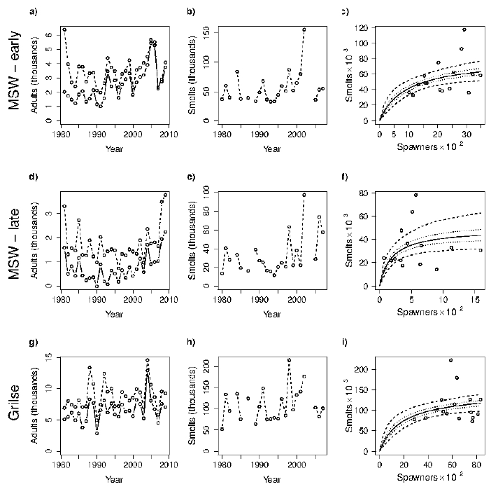
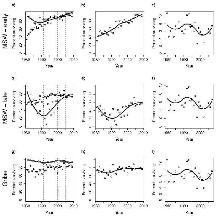
Fig.C.2. Multiple sub-stock survival description for the data not corrected for Grilse-Error fitted with the default allometric marine-marine mortality ( DAM). Compare to main text, Fig.5

Supplement D

Derivation of the equation for obtaining unbiased fish-counter grilse/ MSW ratios despite biased rod-fishery sea-aging returns.

We define E to represent the total escapement from the estuarine net and coble fishery, and note that, since this fishery is unbiased, the ratio of grilse to MSW fish in this escapement is the same as that measured in the samples of fish taken from the net and coble fishery, which we denote by F _N.

Between the net and coble fishery and the resistivity counter in the Logie Burn there is a rod fishery, which extracts a (known) total catch T _RB (where RB denotes "rods below the counter") in which the (known) grilse to MSW ratio is F _RB. The resistivity counter records a "catch" T _C, and we wish to know what value we should assign to its (unknown) grilse to MSW ratio F _C.

To solve this problem we assume that all fish not caught by the rod fishery below the counter are registered by the counter. This amounts to assuming that natural mortality during passage through the rod fishery is negligible and that the counter "sees" all fish passing through it.

Under this assumption the number of grilse seen by the counter is given by

and the number of MSW fish seen by the counter is

These equations contain two unknowns ( E and F _C) so we first eliminate E between the two equations, showing that

which can easily be rearranged to yield a closed form expression for the quantity of interest, namely

Supplement E

Relative fecundity (productivity) ratio calculations between the sub-stocks, across the three marine mortality models and for three ova-productivity metrics.

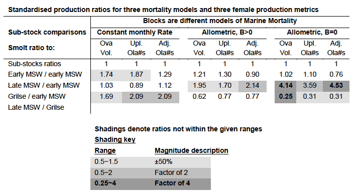
Supplement E illustrates how the fecundity predictions based on the SR analyses of the main paper are robustly compared between the three sub-stocks. It starts by creating 'expectation ratios' for those values, based on information taken from Bacon et al. (2012), as shown in Table E.1. It next (Table E.2) illustrates like calculations based on the SR analyses in the main paper. Tables E.1 and E.2 thus contain ratio estimates of the same qualitative comparisons. Accordingly, if those comparisons, although derived by different approaches, actually estimated the same quantitative values, their joint ratios would always be close to 1.00. Table E.3 (also Table 3 of the main text) presents that final comparison, and shows that most of the resulting 27 ratios ( three sub-stock comparisons * three mortality models * three fecundity metrics) differ from 1.00 very considerably.

Table E.1 Illustrates the calculation of fecundity-expectation ratios between sub-stocks, based on findings in Bacon et al. (2012). The header-column denotes each phenotype or sub-stock-comparison, with the first three rows the phenotypes and the next four their comparison ratios. Thenext, and first numeric, column shows the fork-lengths of typical females. Then, consequent on those fork-lengths and calculated using the equations in Bacon et al (2012), the subsequent columns show: the total volume (mass) of ova produced by such typical females (which is independent of the river-zone they breed in); the numbers of ova expected from such typical females when breeding in the uplands (also the classic expectation from earlier, standard publications, such as Pope (1961); the numbers of expected ova from such typical females when breeding in the lowlands; the final column (river-zone adjusted) is only completed for comparisons between phenotypes.

The final four rows of Table E.1 are the comparison ratios. Their values are obtained by taking the relevant pair of phenotypic sub-stock values in the same column and, depending on the row-header, dividing each numerator by each denominator to obtain the tabulated ratio-value. In the final 'zone-adjusted' column however, the relevant numerators/ denominators are taken from whichever column represents the river-zone in which the phenotype sub-stock would normally breed (thus giving different values to those in the previous two columns).

Observations: North Esk ova-fecundities parameters (based on Bacon et al. 2012)

	Female size Typical fork-length, mm	Total Ova volume, Litres	Ova numbers / female
			Upland Fewer, larger	Lowland More, smaller	zone-adjust
early MSW	725	0.680	5,715	8,274
late MSW	800	0.923	7,206	10,432
Grilse	600	0.378	3,660	5,299
Calculated Ova-Fecundity ratios
early MSW / early MSW	1	1	1	1	1
late MSW / early MSW	1.10	1.36	1.26	1.26	1.83
Grilse / early MSW	0.83	0.56	0.64	0.64	0.51
late MSW / Grilse	1.33	2.44	1.97	1.97	1.97

The first ratio-row of Table E1, early MSW/early MSW is included simply to emphasise that the procedure results in values of 1.00 when the quantities are identical. Only two of the three sub-stock comparison rows are fully statistically independent. However, the third, late MSW/Grilse, is also included as it represents a comparison where the two phenotypes typically breed within the same lowland river-zone, and the comparison thus represents a different biological hypothesis from the other two (in which early MSW which typically breed in the upland river-zone) is the denominator.

Table E.2 Has a similar purpose and overall format (three phenotype rows, four sub-stock comparison rows) to Table E.1. However, its numeric columns represent the values, or ratios, of fecundity estimates obtained from the SR β coefficients estimated from the SR analysis of the main paper. One set of values is tabulated for each of the three marine-mortality sub-models.

Smolts per female from SR β parameter, this paper

Mortality Model	Smolt production per female
	Constant monthly, UR	Default allometric, DAM	Uniform survival, US
Sub-stock	Beta, absolute
Early MSW	124	95.8	92.1
Late MSW	292	157	128
Grilse	70.8	104	212
	Beta, ratios
Early MSW / early MSW	1	1	1
Late MSW / early MSW	2.35	1.64	1.39
Grilse / early MSW	0.57	1.09	2.30
Late MSW / Grilse	4.12	1.51	0.60

Accordingly, both Tables E.1 and E.2 contain fecundity ratios representing the same sub-stock comparisons of relative fecundity obtained from two different numeric estimates of the same qualitative comparison. Thus, if both methods (E.1, from body sizes; E.2 from SR analyses) genuinely reflected the same quantitative values, then the ratio of the estimates (E1/E2) would always closely approximate 1.00. In Table E.3 below it can be seen that this is rarely the case. Table E.3 is identical to Table 3 in the main text, and is reproduced below for convenience, along with some further explanatory remarks.

Table E.3. The table gives a comparative productivity index, calculated between different pairs of sub-stocks, identical productivity estimates via both estimation routes, would always produce an index value of 1.00. The rows show the different pairs of sub-stocks compared. Blocks of three columns show results calculated for three different marine mortality models. Within these triplet-blocks, individual columns show the index as calculated for different productivity metrics (calculated from Bacon et al. 2012 for typically-sized females per sub-stock). Shading and font-style differences (see key) emphasise that none of the marine mortality models produce productivity estimates that are reasonably close to those expected (from female salmon of typical sizes and productivities for the same sub-stocks) across all sub-stock comparisions. Productivity metrics for typically-sized females per sub-stock are: Ova Vol.=total volume of all ova produced per female; Upl.Ova#s=total numbers of ova produced per female in 'upland' river zones (as normally used); Adj.Ova#s= numbers of ova produced per female adjusting for the up-/low-land spawning situations).

Note that ratios differing by only 10 or 20% would imply very large selective advantages. See the main text,and the notes below, for further explanation.

Notes on Table E.3

• Whatever marine-mortality model is used to provide the fecundity estimate ( SR-β), several ratios of SR-β /female_size_expectation are highly disparate from 1.00.
• Although only two comparisons are statistically independent the third, late MSW / grilse, illustrates a different biological assumption regarding the ova-numbers comparison (as both sub-stocks are lowland with the same individual egg volumes).
• The large discrepancies frequently involve the comparison late MSW/grilse where different egg sizes and numbers between river-zones are irrelevant.
• Of the three marine-mortality models here investigated, that for B>0 has fewer and smaller discrepancies, but still has a set of discrepancies that are unbelievably large [1.95, 1.7,2.14].
• The trio of columns representing the 'adjusted-river-zone' ('upland/lowland') comparison of fecundity also has fewer (but still several unbelievable) high values. However, invoking this as an explanation not only still has problems of several high values but also inherently implies a sub-stock difference anyway (due to their segregation between river-zones).
• No marine-mortality model block has a single column (production metric) without at least one highly unacceptable index value.
• The Allometric B>0 marine-mortality model does best overall, but its early MSW/grilse ratios are consistently very poor, and especially so for the OvaVol and Adj.Ova#s, which one might expect would be the more similar index values.
• The Constant Monthly marine mortality model does next well overall (but still badly). Its Grilse/early MSW comparisons are consistently good, but its other comparisons are very bad to extremely bad.
• theAllometric B=0 marine mortality model does extremely badly for most comparisons, with is late MSW /early MSW being least awful.

Supplement F

Multiple sub-stock description for data not corrected for Grilse-Error fitted with the uniform survival marine-mortality model ( US, β _m=0, ). Compare to main text, Fig.4.

Figure F.1 (compare to main text Figure 4). Trends in sub-stock numbers and SR relationships for each of the three sub-stocks, as predicted by the uniform survival marine-mortality model ( US, β _m=0 ). For full legend see Annex Fig.C.1 or main text, Figure 4

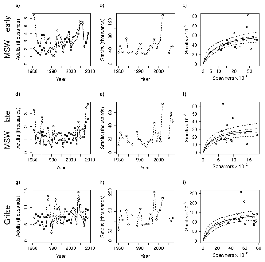
Figure F.2 (compare to main text, Figure 5). Trends in sub-stock survivals for each of the three sub-stocks, as predicted by the uniform survival marine-mortality model ( US, β _m=0 ). For legend see Annex Fig.c.2 or main text, Figure 5.

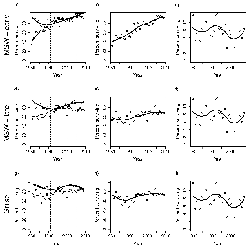
Table F.1 (compare to main text, Table 2). Posterior parameter distribution for the North Esk 1980-2004 spawner to smolt data regarding the system as comprising three sub-stocks, using Beverton Holt ESRs with control priors, as predicted by the uniform survival marine-mortality model model ( US, β _m=0 ) . First two columns show the pair of parameters O _max, H, defining the BH SRcurve-shape. The third column, θ , represents the negative binomial error distribution factor . The next two columns are biologically informative values derived from the former three columns. The fourth column shows the (approx) modal coefficient of error variation implied by θ (see Gurney et al. (2010) equation 2). The fifth column shows maximum individual productivity, β, (equation 8). The top line of each pair shows the mode and lower line shows the upper and lower 95% credibility limits. The upper section of the table shows results for the default (grilse-error corrected) data, while the lower section shows results without grilse-error correction.

Sub-stock	O max mode		H mode		θ mode		CV(%) ≈ 1/√ mode		β = O max/H mode
	2.5%	97.5%	2.5%	97.5%	2.5%	97.5%
Data Corrected for grilse error
MSW early	6.64×10 4		721		8.76		34%		92.1
	5.20×10 4	10.4×10 4	331	2315	4.02	18.3	50%	23%	45	157
MSW late	3.27×10 4		255		3.22		56%		128
	2.40×10 4	5.24×10 4	129	876	1.65	6.82	78%	38%	60	186
Grilse	15.3×10 4		1264		7.96		35%		121
	12.5×10 4	22.2×10 4	589	4012	3.64	16.0	52%	25%	55	212
Data not corrected for grilse error
MSW early	6.67×10 4		758		8.78		34%		88.0
	5.23×10 4	10.3×10 4	334	2266	4.02	18.6	50%	23%	45	157
MSW late	3.43×10 4		159		3.24		56%		216
	2.66×10 4	5.90×10 4	80.2	445	1.58	7.20	80%	37%	133	332
Grilse	15.9×10 4		1330		7.77		36%		120
	12.6× 10 4	22.5× 10 4	639	4487	3.67	16.2	52%	25%	50	197

Supplement G

Multiple sub-stock uniform risk-rate ( UR) marine mortality model ; Graphs and Table.

Figure G.1 (compare to main text Figure 4). Trends in sub-stock numbers and SR relationships for each of the three sub-stocks, as predicted by the uniform risk-rate ( UR) marine-mortality model. For full legend see Annex Fig.C.1 or main text, Figure 4.

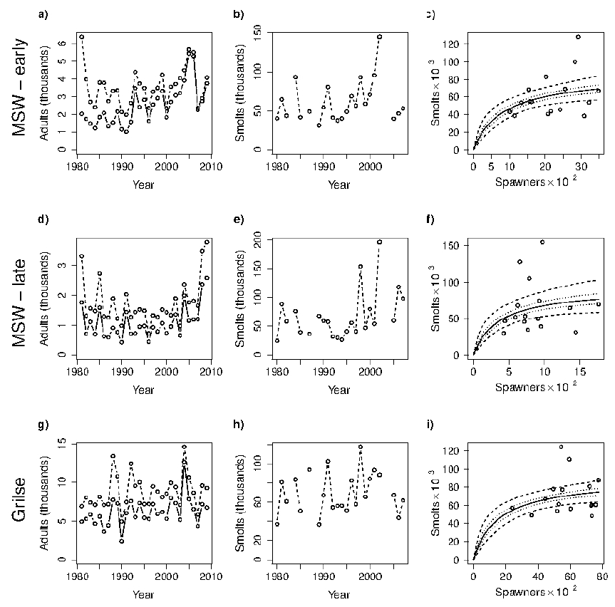
Figure G.2 (compare to main text Figure 5). Trends in sub-stock survivals for each of the three sub-stocks, as predicted by the uniform risk-rate ( UR) marine-mortality model. For full legend see Annex Fig.C.2 or main text, Figure 5.

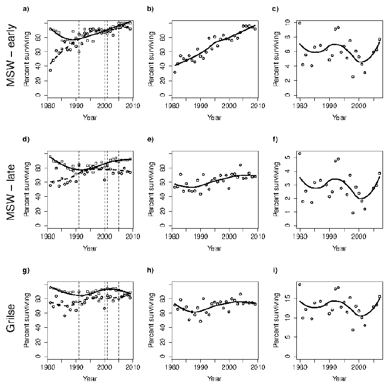
Table G.1 (compare to main text, Table 2). Posterior parameter distribution for the North Esk 1980-2004 spawner to smolt data regarding the system as comprising three sub-stocks, using Beverton Holt ESRs with control priors, as predicted by the uniform risk-rate ( UR) marine-mortality model.First two columns show the pair of parameters O _max, H, defining the BH SRcurve-shape. The third column, θ , represents the negative binomial error distribution factor . The next two columns are biologically informative values derived from the former three columns. The fourth column shows the (approx) modal coefficient of error variation implied by θ (see Gurney et al. (2010) equation 2). The fifth column shows maximum individual productivity, β, (equation 8). The top line of each pair shows the mode and lower line shows the upper and lower 95% credibility limits. The upper section of the table shows results for the default (grilse-error corrected) data, while the lower section shows results without grilse-error correction.

Sub-stock	O max mode		H mode		θ mode		CV(%) ≈ 1/√ mode		β = O max/H mode
	2.5%	97.5%	2.5%	97.5%	2.5%	97.5%
Data Corrected for grilse error
MSW early	7.54×10 4		607		10.92		30%		124
	6.33×10 4	11.1×10 4	272	1628	4.96	21.9	45%	21%	64	253
MSW late	8.06×10 4		276		4.93		45%		292
	6.41×10 4	12.6×10 4	122	781	2.49	10.7	63%	31%	146	584
Grilse	8.67×10 4		1225		15.5		25%		70.8
	7.35×10 4	11.8×10 4	588	3582	6.89	30.9	38%	18%	32	133
Data not corrected for grilse error
MSW early	7.67×10 4		555		10.24		31%		138
	6.34×10 4	11.3×10 4	274	1705	5.05	22.5	44%	21%	64	253
MSW late	8.93×10 4		133		4.60		47		671
	6.86×10 4	13.2×10 4	65.5	331	2.24	11.1	67%	30%	346	1,197
Grilse	8.84×10 4		1446		15.4		25%		61.1
	7.35× 10 4	11.9× 10 4	645	3981	7.05	32.6	38%	18%	28	120

Supplement H

SR curve estimates, including a combined [late MSW and grilse] prediction, based on the default allometric ( DAM) marine-mortality model.

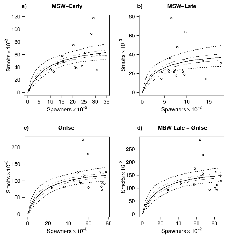
Figure H.1 This figure shows the estimated Stock-Recruitment curves, with the data as points and the credibility limits as dotted lines various sub-stocks, based on the default allometric marine-mortality model ( DAM). Panes a,b,c of this figure are, for ease of comparison, the same as Fig.4.c,f,i in the main text. Pane d of the present figure is a new prediction, produced by assuming that the late MSW and grilse sub-stocks might comprise a single combined stock with the offspring having equal viabilities. For full legend see Annex Fig.c.1 or Fig.4, main text.

Supplement I

Discussion details of 'Reproductive Implications' of the models. N.B. This example is based on the Uniform Risk-Rate marine-mortality model.

We next consider potential causes of these productivity (fecundity) differences. Equation [12] decomposed β into the products of the proportion of the spawning stock which is female (F), the ova fecundity per female (B ₀) and the ova to smolt survival (L _os). To understand these in a wider context one needs to further decompose the ova-fecundity into a female weight W and an ova fecundity per unit female weight B _w, because (certainly at the North Esk), although females of all sub-stocks produce the same biomass of ova per unit of female weight, lowland-breeding salmon (here the late 2 SW' and grilse sub-stocks) produce 45% more-but-smaller eggs from each unit of ova biomass (Bacon et al. 2012). Hence in this extended formulation

Comparing the reproductive capacities of grilse and late 2 SW' pheontypes (whose offspring are generally considered to be co-located in the 'lowlands' ( sensuBacon et al.2012) one can reasonably assume that both L _os and B _ware the same for those two putative sub-stocks.

Hence, to explain the productivity anomaly by different sex ratios, F, given that the female weight ratio is W _LM/W _G=2.5 (see Fig.2) would require, by taking β _G and β _LM from Table 2, and substituting values into a re-arrangement of equation [13], that

This implies that if the late 2 SW' sub-population had a 1 to 1 sex ratio ( F _LM=0.5) one would require the grilse population to have F _G=0.25, equivalent to a male to female ratio of 3 to 1. The North Esk data shows the grilse sub-stock to be some 55% male (a ratio of just 1.2 to 1): so differing sex ratios between the sub-stocks seem an unlikely explanation.

To similarly compare the productivities between grilse and early 2 SW', one takes the appropriate seasonal fish sizes (Fig.2) and allows the numerical ova-fecundity per unit weight, B _w, to be 45% higher for 'lowland' grilse. Hence, in this case, self-consistency of productivity estimates would require that L _EM\L _G= 1.23*(F _G/F _EM). If grilse and early 2 SW' salmon have broadly the same sex ratio (which North Esk data suggest they do) then this suggests that self-consistency would require the ova to smolt survival of early 2 SW' to be some 23% higher than that of (lowland) grilse. Larger ova-volumes (per individual egg) are a very plausible mechanism to achieve such improved survivalin such circumstances (see Einum et al., 2002, Heath et al. (2003), Einum, 2003, Rombough, 2007, van den Berghe and Gross, 1984; Crisp & Carling, 1989, Steen & Quinn, 1999; for details and see Bacon et al. 2012 for an overall, structuring, argument).

Consideration of the likely magnitudes other possible contributory causes to the productivity anomaly between late 2 SW' and grilse (such as the truncated size-distribution of the North Esk grilse and late MSW fish, due to the end of the netting season in autumn seem unlikely to bridge the gap, with the exception of inter-breeding between late MSW and grilse as discussed in the main text.

More detailed discussion of such aspects (which might ultimately depend on habitat 'quality') should probably await more reliable calculations based on more appropriate and realistic models of both marine mortalities, inter-breeding and heritabilities.

Supplement J

Discussion details of 'Fisheries Management Implications'

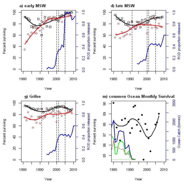
Fig. J.1 The temporal coincidence between estimated North Esk salmon survivals and various fishery pressures. The first three frames show percentage survivals from the estuary nets and river rods; they are labelled (a,d,g) to cross-refer to the like frames of Fig.5, main text . In frames (a,d,g) 'Year' means year of adult return and escapement from/ death due to, the fisheries. Red points and red smoothed fit line show survivals from the estuary nets; black points and black smoothed fit line survival from rods; the blue line shows the recorded change in the proportion of rod-caught salmon that were also released alive. Note the different patterns of rod-release early and late in the season [ (a) versus (d and g)]. Vertical dotted lines are the times of the main fishery management actions (see legend Fig.5). Frame (m) shows the estimate percentage monthly oceanic survival, common to all sub-stocks, as black points with a black smoothed fit line. Note the very different survival scale for frame (m) compared to (a,d,g). In frame (m) 'Year' is the year of smolting for each cohort. The coloured lines are oceanic fishery takes in tonnes, offset to reflect the appropriate years the cohorts were at sea. Blue is total oceanic take; solid green the take at West Greenland; dotted green the take at East Greenland; dashed red the take at Faroes.

Mangement Implications; Marine fisheries, Scottish Fisheries and Conservation Limits

J.1 Marine Fisheries

The constrained nature of the marine mortality model necessarily used here, combined with the influential marine survival estimate for the 1980 cohort (Fig.s 5, J.1) make it very hard to see any effect on survival of the declining oceanic fishery catches between 1980 and 1994. Despite high tonnages of ocean catches in that period (Fig.J.1.m) it seems likely that the expected beneficial effects are masked by the high year-on-year variability and the evident large underlying fluctuations of natural mortality processes. Note especially that fluctuations in estimated marine mortality subsequent to 1990 (Fig.J.1.m), when oceanic fisheries were very low to absent, show fluctuations from unknown causes that were of similar magnitude to those seen between 1980 to 1990 (when the oceanic fisheries declined); there is no reason to believe that these other unknown causes would not have been acting from 1980 to 1990, further complicating the ability to discriminate potential causes.

J.2. In-River Fishery Management

Local fisheries management actions at the North Esk were aimed mainly at the early MSW stock, so it was not unexpected to see no evident effect of those actions on the grilse or late MSW sub-stocks. Fig.5.b provides an encouraging message for the conservation of the North Esk's early-run MSW salmon, namely that in-river fishing mortalityhas decreased steadily from 60% to under 5% between 1980 and 2009.

However, the message is less clear concerning the relative merits of specific management actions to aid early MSW salmon. Early MSW survivals from both the nets and the rods (Fig.s 4.a,5.a) were well underway before either the formal delays to the netting season or the recorded introduction of rod catch-and-release around 2001 and 2005 (Fig.4.a) and marked increases in C&R do no show clear responses in survival (Fig.5.a). Nor does the pattern of late-season C&R closely match estimated survival changes (Fig.5.d,g). However, discerning the benefits from those formal management actions (net season delay, C&R) was inevitably constrained by the already high survivals (around 80%, Fig.s.4,5), and any sudden improvements could have been masked by annual variation in the estimated survivals. Moreover, that masking has probably been exacerbated by lack of detail on other potential causal factors, such as fishing effort (both net and rod) and other environmental factors affecting fishes' catchabilities. Nevertheless there is now nearly complete escapement for early MSW salmon, a situation which could not have arisen with the former levels of takes from the fisheries.

J.3. Conservation Limit ( CL) 'Parameter Transportation' Considerations

The key population parameters that are frequently outside the knowledge and control of the local fishery managers (who monitor and\or control the in-river takes by different fishery methods) are the spawner-to-smolt SR production and the marine mortality ^[3] .

Overall understanding of marine mortality is severely constrained, but with scant evidence of any large or well understood local (river-to-river) effects (eg Chaput 2012). So there is little option but to transfer the widely-differing overall (smolt to PEA) survivals for the different sub-stocks ^[4] .

Transferring the information about the (deterministic) SR relationships is aided by reference to the productivity values, β (see Eqn.7, main text). The SR β reflects both the average fecundity of individual spawning fish of the sub-stock of interest (which could rather plausibly be assumed not to vary greatly between catchments within sub-stocks) and, secondly, the survival from spawner to smolt at low (fry) density. As a first approximation in the absence of appropriate 'habitat' information, then at low densities, that survival might plausibly be viewed as reasonably constant ^[5] .

The maximum smolt productivity ( O _max) for a given sub-stock in a given catchment almost axiomatically scales with the ratio of the amount of suitable habitat for the given sub-stock between the two catchments (eg Chaput 2012). However, as the habitat requirements for both redds and juvenile salmon (l et alone the important finer details of their spatial distribution, such as whether there are many (small) adjacent patches of each, or not) are quite complex, the central problem would seem to be measuring the quality and quantity of available habitat in the donor and recipient rivers. Investigation of the use of simple river-catchment- or wetted-surface-area ratio metrics in Scotland have met with mixed success (MacLean 2007).

The considerations discussed above suggest that the present lack of knowledge about 'extent of suitable habitats' in different rivers may well be the biggest constraint on transferring (sub-stock or any other) population parameters from 'donor' to 'recipient' catchments. If so, this suggests that a modest amount of well-targeted additional research will be needed to determine a set of broad environmental parameters which, together, define an aggregated `habitat measure' and thus allow the re-scaling of maximum smolt productivity ( O _max) between rivers. While such work is likely to concentrate on environmental parameters readily determined by GIS methods, it seems probable that inter-catchment comparisons will play a vital role. Accordingly, if the presumed 'generality' of such smolt production estimates across rivers (and its relationship to habitat metrics) is to move from being an act of faith to one established by data, then suitable fish population data will also be needed from several rivers. Given the presently small number of catchments for which appropriate salmon population data exists to enable such comparisons (currently only three in Scotland), this reasoning reinforces the views of Chaput (2012) that a more carefully targeted approach to the collection of population data is a key future management requirement for Atlantic salmon. Once an effective aggregate 'habitat' measure has been defined (probably involving environmental metrics such as water quality and temperature as well as remotely-sensed river-water characteristics), and collated in a GIS framework, then inter-catchment transfer of relevant population parameters for phenotypically homogeneous sub-stocks of Atlantic salmon could become both more reliable and routine.