Passive acoustic monitoring as a tool for offshore wind farm biodiversity assessments: a pilot study

3. Methods

3.1 Study sites

Passive acoustic monitoring metadata from 332 moorings provided by the Marine Directorate were screened for the presence of calibration information and broadband acoustic data. From the latter, 200 moorings were identified as having broadband and calibration data originating from 20 different locations. For the purpose of this pilot study, and to maximise the amount of data from contrasting habitat types while minimising the effect of seasons and interannual changes on the soundscape, the available datasets were searched for the year in which most sites had data collected in April. April was chosen as this is when key fish species are likely to spawn in Scottish waters (FishBase, 2024) and the effect of wind on the ambient noise would be reduced (De Clippele and Risch 2021).

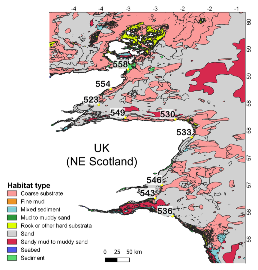
The centre frequency 1/3 Octave Band Sound Pressure Level (SPLrms) were then calculated using PAMGuide (Merchant et al. 2015) to determine which day in April was the least affected by wind and anthropogenic noise pollution. The PAM data collected in April 2021 included most sites (datasets), 18 in total. The 100 Hz (SPLrms) data was plotted using ggplot in R version 4.0.0 and revealed that 23^rd of April was the most suitable day for further analysis, as it had the least amount of ambient noise at the 100 Hz frequency band (Supplementary Materials, SM1). However, one of the locations, Arbroath site, only had data available until the 12^th of April. To avoid reducing the number of sites for analysis, the 10th of April was identified as the second most suitable day. Visual inspection of historical weather data on Visual Crossing (Visual Crossing, 2024) revealed that the noise levels were predominantly driven by wind gust strength at the sites. Inspection of the acoustic data from the Latheron site, confirmed that the peak in SPL (up to ~130 dB re 1 µPa of the 1/3 Octave band) was related to ship activity very near the site (SM1). Of the 18 moorings sites reviewed, nine were used for further analysis as sharing permissions were in place during the duration of the project (Figure 1). One of the locations, Duncansby Head (Deployment no 558), was heavily polluted with artificial mooring noise and was therefore also excluded, leaving eight sites in total (Table 2).

3.2 Environmental data

To understand what biological and environmental variables contribute to explaining spatial differences in the soundscape, Geographic Information System (GIS) layers were downloaded from open-source platforms and imported into QGIS (version 3.4.13, QGIS, 2024). An overview of the data and their web links are provided in the supplementary materials (SM2), and include, depth, the EUNIS (European Nature Information System) habitat type (Figure 1), temperature, current speed, primary productivity, and dissolved organic carbon. The QGIS spatial analyst tool (Extract Multi Values to Point tool) was used to extract the environmental information from the sites for statistical analysis.

3.3 Biodiversity data from open-source platforms

Benthic biodiversity data were downloaded from the OneBenthic portal (Cooper and Barry 2017, 2020). The OneBenthic data is a map of 12 different faunal clusters, based on classifications from random forest models of environmental data and seabed core and sediment samples (Cooper and Barry 2017, 2020). Each faunal cluster is associated with an assemblage of likely taxa that would be found in each area. At each mooring location, the OneBenthic faunal cluster species richness and faunal cluster category, alongside the area (km²) of the faunal cluster occupied at the mooring location were extracted and used as additional variables for statistical analysis.

The area that an animal will use to feed, i.e. their home range, is species dependent. While some species, such as the European Lobster, have a home range smaller than 5 km (Smith et al. 2001), fish such as cod may travel a distance of 15 km to find food (Neat et al. 2006). The number of faunal clusters present within an intermediate home range area of 10 km radius, was therefore extracted, as a higher diversity of habitats present in an area may affect species presence. This variable is here referred as “Habitat complexity”. This radius was chosen based on the assumption that species of interest may travel in these areas, but it is important to note that their vocalisations may not. For example, sounds produced by cod may travel around 400 m (Seri et al. 2023). The OneBenthic faunal cluster categories are also solely based on invertebrates, for which soniferous behaviour is largely unknown or unlikely (Parsons et al. 2022; Looby et al. 2023). The number of species which use our sites as essential spawning or nursery fish habitats were extracted from essential fish habitat (Franco et al. 2022) and fisheries sensitivity maps (Marine Scotland 2022). As part of these maps, areas are categorised as “absent”, “low”, and “high” for certain fish species. Since numerical data was needed for analysis, here the sum of the species, which were categorised as “high”, were counted.

To determine if and which soniferous species may be present in the area surrounding the study sites, species available per a location’s 10 km² radius (see above’s justification) were downloaded from the National Biodiversity Network (NBN) Atlas (NBN Trust 2024). The NBN Atlas contains species occurrence data submitted by trusted organisations and recorders and collated, integrated and standardised by the NBN Trust (2024). The extracted NBN data was screened to ensure only relevant marine species were included. Records from museums, historical surveys, non-animal and non-marine were excluded. Due to shifting species ranges, as a result of changing sea temperatures, only records from 2014 onwards were kept.

This list was compared against a recently published global inventory of species confirmed or expected to produce sound underwater as part of a collaboration between the Global Library of Underwater Biological Sounds (GLUBS) with the World Register of Marine Species (WoRMS) (Looby et al. 2023) and fishsounds.net. The GLUBS database uses species lists from WoRMS and assigns species to one of six categories denoting knowledge of sonifery. A further literature search was then conducted to detail any available acoustic characteristics of sounds made by soniferous species. If open-access sounds were available, available information on sound type, peak frequency and duration of the sound were recorded.

3.4 Passive Acoustic Data

All recordings had a sampling rate of 96 kHz. All acoustic files were visually and auditorily screened in the software Raven Pro (version 1.6). The noise produced by vessels, the moorings, or pile driving were categorised as anthropogenic. Distinct anthropogenic noises such as pile driving, self or vessel noise were annotated in Raven with bounding boxes. These selections were then removed using the delete tool within Raven Pro, to further test if noise pollution affects acoustic index values (Zhang et al. 2024). Any biological sounds which may have been masked by this anthropogenic noise would also have been removed. Four subsamples of ten-minute continuous recordings were selected per site, around sunset, midnight, sunrise and midday. Based on historical data, sunrise happened at 06:16 and sunset happened at 20:08 on 10/04/2021; with the exception of St Abbs at dawn, these times appeared clear of shipping noise pollution. Due to slight differences in the timings of recordings at each site, the four selected were the first after sunrise, the last before sunset, and the closest to both solar midday and midnight (SM3).

3.4.1 Acoustic Community, Phonic Richness and abundance

Biologically produced sounds were manually annotated in Raven Pro version 1.6. For the purpose of this study, both active and passive sounds were considered, which resulted in the acoustic community and phonic richness data. Due to the typical low frequency content of fish sounds, the Raven Pro spectrogram was explored up to 4 kHz. Sounds which had a frequency range higher than 4 kHz were also annotated when they were visible in the lower frequency ranges (< 4kHz), as some benthic invertebrate sounds can extend to around 10 kHz. The x-axis was zoomed to ~12 seconds, to give enough detail to clearly label the start and end of specific acoustic events. Sounds were labelled and counted and a datasheet was created containing information on the number of different type of sounds per subsample. The phonic richness was calculated as the total number of types of sounds per 10 minute sample. To determine if the sounds were active or passive sounds, the envelope of the sounds were investigated by a fish bioacoustic expert. Detailed characterisation of the different sounds types is out of the scope of this report.

3.4.2 Acoustic indices

A total of seven acoustic indices (Table 1) were calculated (Sueur et al. 2014). To calculate the acoustic indices, each selected recording was filtered using a short-term Fourier transform band-pass filter into different frequency bands at the low-frequency band (50 – 1,000 Hz), a relatively higher frequency band (1,000 – 2,000 Hz) and this frequency band as a whole (20 – 2,000 Hz). The chosen range of the different frequency bands was based on the frequency bounds of the annotated types of sounds and to avoid impacts of marine mammal sounds. While peak frequency bands of some invertebrate sounds may not be included in this range, their sounds usually extend to the lower frequency ranges as well. As mentioned above, only sounds extending below 4 kHz were annotated. The indices were calculated in R using the packages seewave (Sueur et al. 2008) and soundecology (Villanueva-Rivera and Pijanowski 2018). Acoustic indices were calculated for both the raw and cleaned audio files, i.e. after mooring and anthropogenic noise were removed.

3.5 Statistical analysis

To determine what drives the differences between the acoustic communities, first, the acoustic community data were Hellinger transformed using the decostand function in the vegan package (Oksanen et al. 2017). A Hellinger transformation was used to convert sound type abundance values to relative values, to address absences of certain types of sounds across multiple samples. Then, the Bray–Curtis dissimilarity measure was computed with the vegdist function. This measure calculates the dissimilarity between two samples based on the relative abundances of species present in those samples (Oksanen et al. 2017). To test if the acoustic communities significantly differ in relation to the OneBenthic faunal cluster type and the habitat type groups an analysis of similarity (ANOSIM) was conducted using the Bray-Curtis dissimilarity matrix. ANOSIM compares the mean of ranked dissimilarities between groups to the mean of ranked dissimilarities within groups. This was followed by a permutational analysis of variance (PERMANOVA) to test the magnitude of the dissimilarities, using the adonis2 function. This allowed to test if the patterns of variation in composition and in abundance of types of sounds in relation to faunal cluster and habitat type were different. If differences were found using ANOSIM, then similarity percentages (SIMPER) analysis was used to identify which types of sounds primarily accounted for observed differences in soundscape assemblages between faunal clusters and habitat types. This method does this by calculating the average percentage contribution of each variable to the overall Bray-Curtis dissimilarity between the chosen groups.

This was followed by the development of multivariate redundancy analysis (RDA) models to establish which variables contributed to explaining differences in the acoustic communities. The explanatory variables (i.e. depth, temperature, current speed, primary productivity, dissolved organic carbon, substrate, OneBenthic richness, Area of the OneBenthic class, and the number of species that use the area as a nursery or for spawning) were normalised using the decostand function in the vegan package. This function makes the margin sum of squares equal to one (default margin is 1) (Oksanen et al. 2017). To determine which explanatory variables were statistically important, forward selection was conducted using the ordistep function. The selected variables were then used in a partial RDA model, constraining the variables that are not metrics representative of the benthic biodiversity.

Correlation and Kruskal-Wallis tests were furthermore used to test correlations between metrics and differences between habitat types and faunal clusters. To test correlations between the habitat types and the acoustic indices, the habitat types were categorised, with “2” indicating hard substrates and “1” indicating sandy substrates.