Passive acoustic monitoring as a tool for offshore wind farm biodiversity assessments: a pilot study

4. Results

4.1 Benthic biodiversity

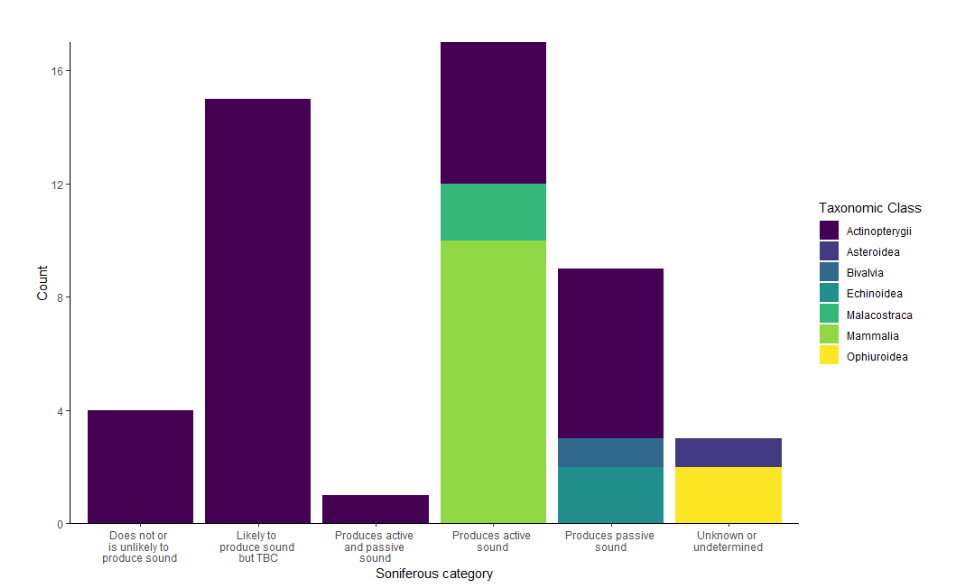
The data extracted from the NBN database resulted in a total of 5,615 records belonging to 482 different species, extracted from the 10 km² buffer area around the location of the mooring sites. The species list from NBN Atlas across all eight sites was combined with the publicly available sonifery information from the GLUBS database. Of the 482 species recorded in the NBN data, 49 species had been assessed in the GLUBS database (Parsons et al. 2022; Looby et al. 2023). Details of the soniferous categories and numbers of species in different taxonomic groups are presented in Table 3, Figure 2 (see Data Availability). Of the 433 species not featured in the database, 417 were invertebrates, which are understudied in terms of the sounds they produce, so should be treated as “unknown or undetermined”. Other species that were not assessed were two Elasmobrachii (shark) species and 14 Actinopterygii (ray-finned fish) species. The full list of species found in the buffer area includes invertebrate and vertebrate species, as well as all species included in Marine Scotland’s Essential Fish Habitat reports (Franco et al. 2022), some of which were not recorded in the NBN records. Because the NBN records are not collected in a standardised manner, this data is not used in the analysis but is used as contextual information.

A total of four PAM moorings were located within “coarse” sediment habitat types (i.e. Spey Bay, Latheron, Fraserburgh, St Andrews), one in “rock or hard” substrate (i.e. St Abbs) and three within “sandy” habitat types (i.e. Cruden Bay, Arbroath, Helmsdale) (Table 4, SM4). The coarse and hard substrate categories were merged as “hard substrates” for further analysis. The depth of the moorings ranged from 21-48 m depth, with Arbroath (47 m) and Helmsdale (48 m) being the deepest sites, and Spey Bay (23 m) and Cruden Bay (21 m) being the shallowest sites. Only three benthic faunal clusters were found to be associated with the study locations, i.e. D2a, D2b and D2c. According to Cooper and Barry (2017) the D2a assemblages are found in areas with more mixed sediments, while assemblages associated with D2b and D2c are found associated with deeper water and are assumed to be largely stable through time. The D2b assemblage is found in areas of high mud content with weaker currents and D2c dominates in areas of higher sand content. Polychaetes were the dominant faunal group across the assemblages, with bivalve molluscs being a feature of group D2b. D2c has the lowest mean number of taxa and abundances associated with faunal groups (Table 4).

The faunal cluster’s habitat size underneath the moorings located at Helmsdale, St Andrews and Cruden Bay were the largest. The “complexity”, i.e. the number of different classes found per mooring site, within a 10 km² radius is shown in the Supplementary Materials (SM4). The most complex site was St Andrews, with 6 faunal cluster classes ranging from 1.25 km² to 154.45 km² in patch size. The least complex sites were Latheron and Fraserburgh, each only having 3 benthic classes present, although both of these sites were in the bottom four for sea surface area within the 10 km² buffer. This is because they were located close to land, meaning that some of the 10 km² overlapped with land rather than the sea. All other sites had 5 classes present, though many had less than 0.5 km² of some classes. It is noteworthy that all sites, except Helmsdale were located within 10 km from land meaning that part of their 10 km² buffer zone did not contain any benthic classes.

Some of the locations were categorised as potential spawning grounds for cod, plaice, sandeel and whiting, and nursery areas for cod, spurdog, Blue Whiting, Tope Shark, herring, Hake, ling, mackerel, anglerfish, plaice, sandeel and Spotted Ray (Franco et al. 2022). An overview of which species were listed to use each of our study locations as a spawning or nursery habitat can be provided upon request (See Data Availability).

4.2 Acoustic Community

In total, 2,592 individual sounds were labelled across the 310 minutes of audio examined. These sounds were labelled as 16 different types of sounds, likely including both passive and active sounds (Table 5). Spey Bay and St Andrews have the highest abundance of sounds across the four 10-minute samples. Two types of sounds were characterised by acoustic features similar to those previously reported for communicative fish sounds (Desiderà et al. 2019; Bolgan et al. 2022; Raick et al. 2023b); these were labelled “thump” and “drum”. Thump was recorded in Arbroath, Spey Bay, St Abbs and St Andrews, while Drum was only recorded Spey Bay (Table 5). “Thump” can be described as a complex sound made of two components; a pulsed component followed by a frequency-modulated component. Its total abundance was highest at St Andrews. “Drum” can be described as a pulse series and was present only at Spey Bay. The types of sounds “whoop”, “tap”, “sneeze”, “whew”, and “plop” were either fish or invertebrate active or passive sounds, while the others, such as “tick”, “grunt”, “scrape”, “crackle”, “click”, “squeak”, “snap” and “chirp” were either invertebrate or passive fish sounds (Table 5). More information on their acoustic characteristics can be found in the supplementary materials (SM5).

The acoustic community data exhibited distinct clusters depending on the habitat type (i.e. hard vs sandy habitats) (ANOSIM: R: 0.1426, p-value < 0.02) and faunal cluster type (i.e. D2a,b,c) (ANOSIM: R = 0.12, p-value = 0.05). There was a significant interaction of faunal cluster and habitat type (PERMANOVA; F= 3.1173, p-value = 0.002). The cumulative contribution of the most influential types of sounds between hard and sandy substrates were “thump” (73%), “tick” (63%) and “grunt” (52%) with “thump” and “grunt” being higher in hard substrates, and grunt being higher in sandy habitats. “Thump” and “crackle” explain the majority of the dissimilarity between D2b and D2a (ST1: 74.85% and ST7: 67.76%) and, “grunt” and “thump” between D2b and D2c (ST3: 79.61% and ST1: 68.00%). “Whoop” (74.34%) and “thump” (68.22%) are the other two types of sounds which are most different between D2b and D2a. “Thump” and “tick” were on average highest in D2c, “grunt” was on average highest in D2a, although only one site was associated with this faunal cluster. “Whoop” was only present in D2a (Table 5). 23

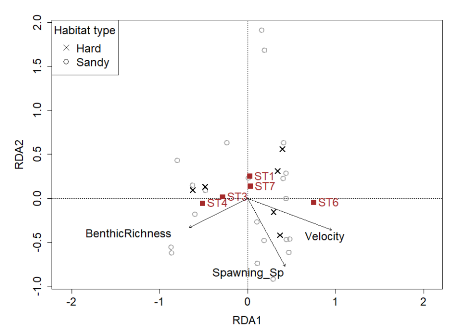
An RDA was conducted to establish which environmental and biodiversity variables drive differences in the acoustic communities (i.e. based on abundance data of the different types of sounds) associated with each of the samples (Figure 3). Collinearity was reduced by removing variables with strong correlations (>0.8), while keeping the variables that explain the most variability in the data. Benthic richness, velocity, and the number of spawning species were kept in the final model. The model explained 27% of the variation in the acoustic communities. A partial RDA, constraining velocity, showed that the benthic biodiversity variables (i.e. NBN benthic richness and number of spawning species) accounted for 17% of the variation, while velocity accounted for 9%. A total of 73% of the variability remains unexplained. ST6 “tap”, ST1 “thump”, ST7 “crackle”, ST4 “scrape” and ST3 “grunt” were the top five sounds driving differences between the different communities.

Removing noise pollution from recordings resulted in files of different lengths (SM3). Latheron, Arbroath and Fraserburgh had the highest occurrence of anthropogenic noise, based on the removal of distinct anthropogenic noise events. Helmsdale was the least noise-polluted site, with only one second being removed on average. The dawn recording from St Abbs was listened to, however no sounds were labelled due to loud boat noise masking all other audio in this recording.

4.3 Phonic Richness

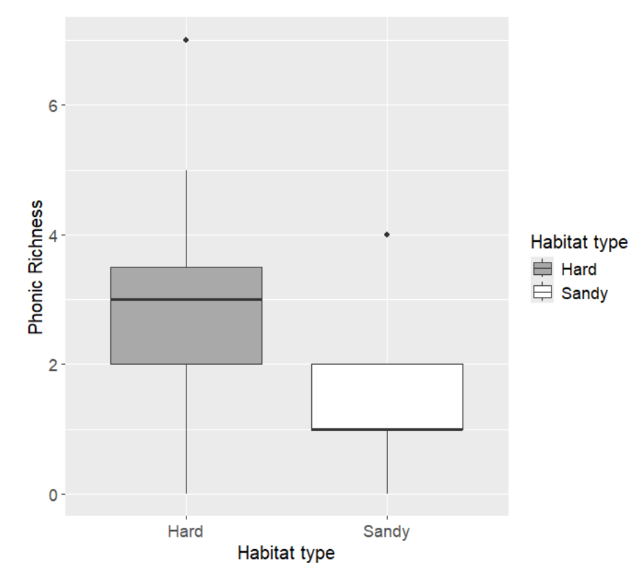
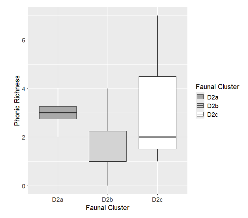
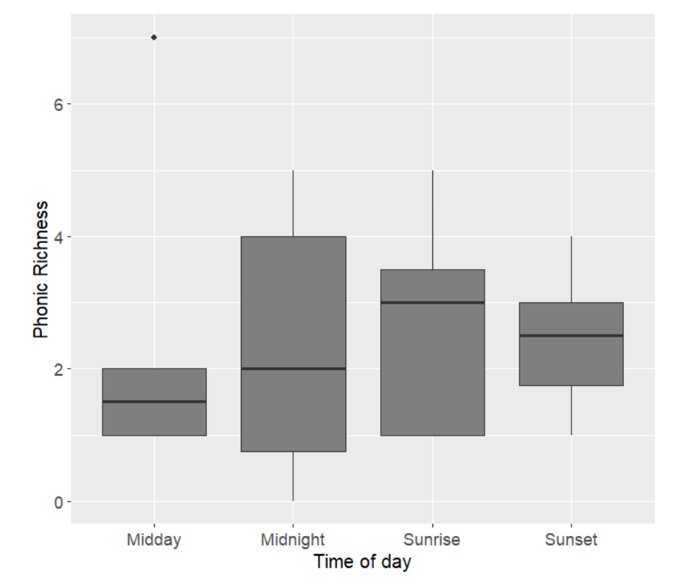
Spey Bay, Latheron and St Andrews had the highest richness of types of sounds (Table 5). Overall, the phonic richness (PR) was significantly higher in areas with coarse/hard EUNIS habitat types, compared to sandy EUNIS habitat types (Kruskall-Wallis test, p-value = 0.03; Figure 4). When comparing the PR between the benthic faunal clusters, no significant differences were found (Figure 5). PR at sunrise and sunset tended to be higher compared to midday and midnight, although no significant differences between time of the day could be found, likely due to the lack of temporal replicates per site (Figure 6). A negative relation (p-value <0.05) between phonic and benthic richness was found (correlation: -0.30), although this was not significant.

4.4 Acoustic Indices

Three of the acoustic indices (definitions and acronyms are explained in Table 1) were correlated with benthic richness, i.e. ACI, AEI and M (Table 6). Higher benthic richness values were correlated to a higher acoustic complexity index, a lower unevenness between frequency bands and to quieter recordings (Table 6).

A total of five acoustic indices were correlated to habitat type and phonic richness, i.e. BI, H, TE, SE, and M. Harder substrates were correlated to more even signals as a whole, but not across time bands within the recordings. Harder substrates are also related to louder recordings, but a lower variability across frequency bands. Since phonic richness is correlated to harder substrates, the acoustic indices follow a similar pattern (Table 6)

Table 6. Overview of the relationships between the traditional metrics of benthic habitats and the computational acoustic metrics.

OneBenthic Richness

Habitat type (i.e. hard vs soft sediments)

Phonic Richness

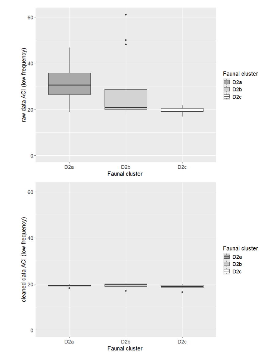
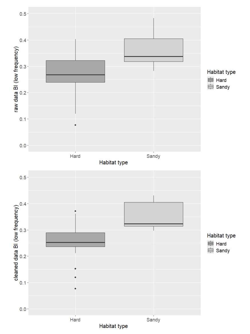
The above-mentioned indices, calculated from the cleaned data, were compared with those calculated from the raw data to test if they produced different results. No overall significant differences were found when comparing the index values with each other. However, this doesn’t rule out that the acoustic index values can be drastically different for a file which has anthropogenic noise removed. For example, in Figure 7 it can be observed that the ACI for the D2a faunal cluster is much higher in the cleaned (ACI: ~30) vs the uncleaned data (ACO: ~20), while in Figure 8 no difference was observed for the BI values related to hard and sandy habitat types.