Decarbonising heating - economic impact: report

Appendix D FTT:Heat - Simulating the effect of policies

FTT:Heat approaches technological diffusion from a non-equilibrium, bottom-up simulation perspective. In the FTT philosophy, agents ground their technology decisions – in this case boiler types – on perceived costs but they do so with bounded rationality (i.e. imperfect knowledge, imperfect foresight, constrained access to information) while not discarding inertia, habits, and loyalty (McCollum, et al. 2017). This approach is significantly different from the economic philosophies used in most IAMs. Other models assume fully rational utility or profit maximising agents with perfect foresight and unbounded access to information.

While the economic philosophy behind the models employed by Cambridge Econometrics is different from the mainstream, there is use for them and the output is valued by policymakers. For example, FTT:Heat has roots in providing insights to European policymakers (Knobloch, Mercure and Pollitt, et al. 2017), and has subsequently been applied to decarbonisation scenarios on an East Asian (Knobloch, Chewpreecha, et al. 2019) and global scale (Knobloch, Pollitt, et al. 2018) as well. With adaption, FTT:Heat has provided scenario-based analysis for the decarbonisation of the Scottish heat supply.

An economic agent in FTT:Heat can choose to replace their heating technology when the existing one reaches their end of lifetime (EoL) or prematurely if an alternative heating technology meets a certain payback threshold.

D.1 End-of-Lifetime replacements

We will first turn to EoL replacements. The FTT methodology of estimating agent's decision-making was developed by Mercure (2012). The mathematical framework for FTT:Heat will be repeated here. First, the net present value (NPV) of the utility (providing heat) for each boiler type is estimated. See Eq.1.

Levelised cost of heat

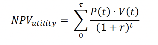
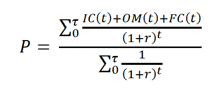
Where: P is the unit price of useful heat (alternatively, the perceived value of utility); V is the requirement for heat (equal to 1 unit of useful heat provided); r is the discount rate; and τ is the lifetime of the technology.

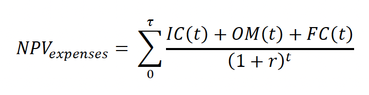
Where: IC is the investment cost component; OM is the repair and maintenance cost component; and FC is the energy cost component.

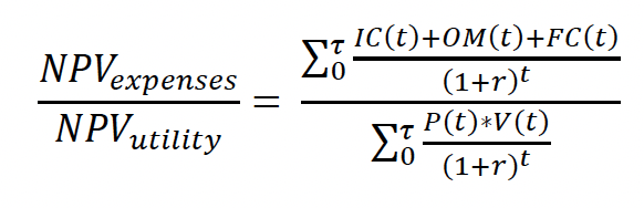
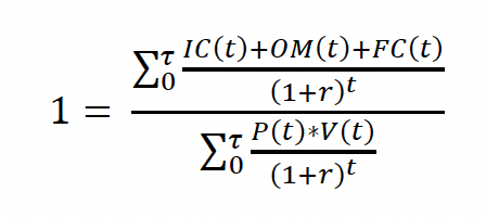
Using the NPV estimates for expenses and utility, a break-even cost can be calculated. This is done by first dividing the NPV of the expenses by the NPV of the utility as depicted in Eq.3. If this ratio is set to equal 1, then the break-even point between discounted expenses and discounted utility can be estimated.

If we assume sales prices, P(t), remain constant over the lifetime of the technology, then this can be extracted from the summation.^[9] While prices fluctuate over time, it is reasonable for consumers to assume constant prices due to imperfect market foresight. See Eq.5 (note that V(t) equals 1, as we are considering 1 unit). This price is also referred to as the levelised cost (LC), see Eq.6. The breakeven price is referred to as such throughout this document.

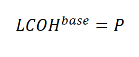
Where: LCOH^baseis the levelised cost without calibration.

The LCOH^base only covers real costs (e.g. investment costs, fuel costs, etc.) and no intangible 'costs'. Intangible costs can be anything from the perception that renewable heating technologies are unreliable to already having a connection to the gas grid which makes a gas-based option more attractive. They include habits and loyalty. In addition, gamma values also cover data gaps.

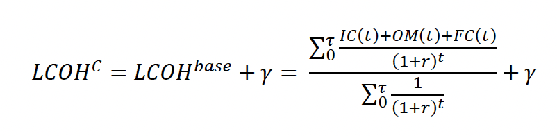
Where: LCOH^c is the calibrated levelised cost; and is the gamma value to calibrate the levelised costs to match historical trends.

However, the levelised costs are not perfectly defined due to local variations (Mercure 2012). Moreover, investors and consumers may have different perceptions and valuation of future costs, i.e., consumers are heterogeneous in their behaviour and decision-making. For these reasons, the cost categories are assumed to be distributions, and therefore the LCOH will be distributed as well. Its standard deviation is then given by Eq.8

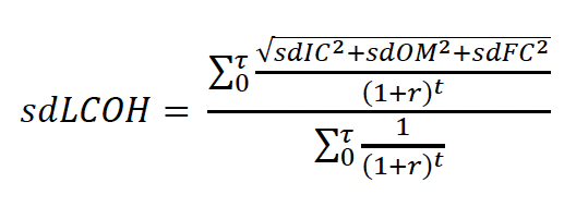
Where: sdLCOH is the standard deviation of LCOH, and sdxx is the standard deviation of the respective cost components. Note that this assumes that the covariance between the cost categories is zero.

The mean and standard deviation of the LCOH are calculated for every technology option and serve as inputs for the EoL decision making core. Technologies are compared on a pair-wise basis and the decision making is based on the construction of binary logits (see Eq.9 and Eq.10).

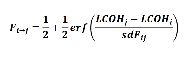
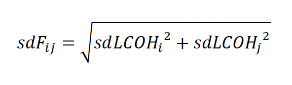
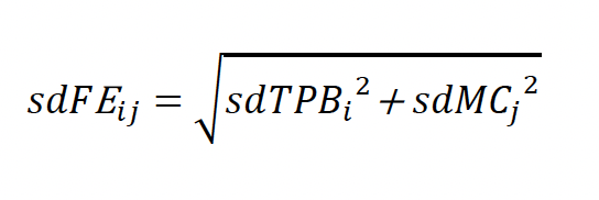
Where: F represents EoL replacement preferences; erf() indicates the error response function; LCOH indicates the mean of the levelised cost; and sdF_ij indicates the standard deviation of preference, which is a function of the standard deviation of the LCOHs of both technologies (see Eq.11 below).

Eq.12 and Eq.13 below are equivalent to Eq.9 and Eq.10; they are rewritten to align with variable notation used in Figure A.1.

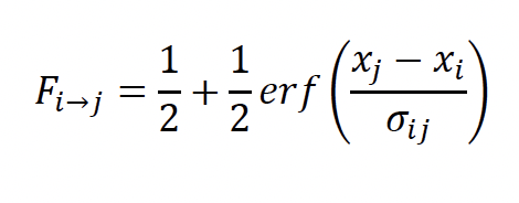
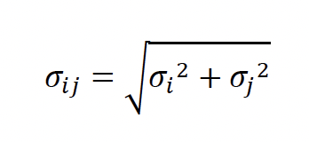
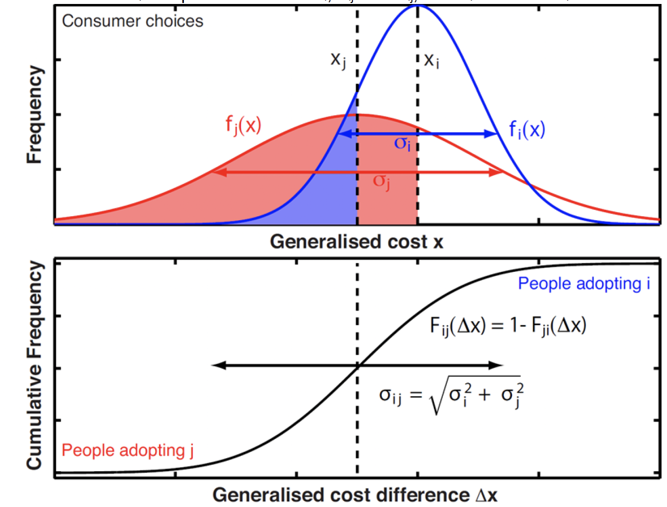
Notes: Illustration of consumer preferences when presented with two choices. Top panel shows the LCOH distributions of two technology options (𝑖 and j, with their respective mean, 𝑥, and standard distribution, σ). Bottom panel illustrates the binary logit as a function of the cost differences. The width of the binary logit is determined by the standard deviation of the preferences (σij). Courtesy to Jean-Francois Mercure and Florian Knobloch.

Figure D.1: Illustration of consumer preferences when presented with two choices.

An illustration of different cost distributions of technologies and how this leads to the construction of a binary logit is illustrated in Figure D.1. The top panel shows the mean and standard deviation of two technology types. The bulk of the consumers will perceive that technology j is cheaper than technology i. Yet, for some the perceptions or local conditions may be such that technology j is (or is perceived as) more expensive than i.

D.2 Premature replacements

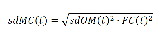
Now, we turn our attention to consumer preferences to prematurely replace the existing heating technology. This is estimated by comparing the marginal cost (MC) of the existing technology to the "Total pay-back cost" (TPB) of an alternative technology. The MC of each heating technology is calculated as depicted in Eq.14 and the standard deviation in Eq.15.

Marginal costs of heat

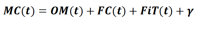
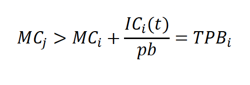
When the difference of the marginal costs between the existing and an alternative technology over the whole pay-back threshold is greater than the investment of the alternative technology, then the consumer may choose to prematurely replace its existing technology. This is depicted in Eq.16.

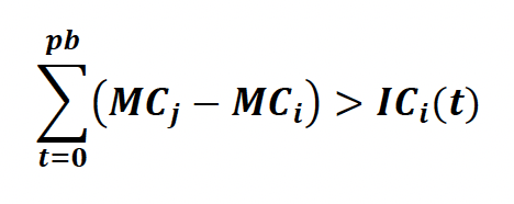
Where: pb is the pay-back threshold.

The consumer will likely assume that the marginal costs for both technologies will remain constant over the pay-back threshold. In that case we can rewrite Eq.15 to Eq.16 which provides an estimate for the Total pay-back costs (TPB).

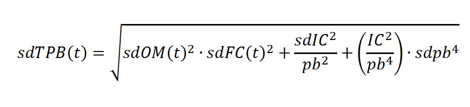
The standard deviation associated with TPB is given in Eq.18.

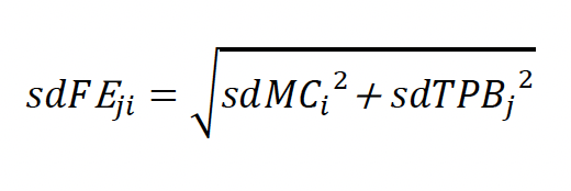
Premature replacement preferences are calculated in a similar way to the EoL replacement preferences. See Eq.19 and Eq.20. A binary logit is constructed based on pair-wise comparisons of marginal costs and Total pay-back costs. Unlike the EoL replacement preferences, the premature replacement preferences of consumers adopting technology i and the premature replacement preferences of consumers adopting j do not have to add up to 1. The calculation allows for no premature replacements to occur at all as it is possible that the marginal costs of the existing technology is lower than the Total pay-back costs of all the alternatives.

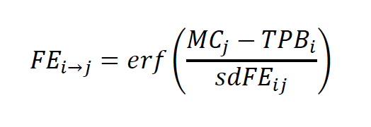
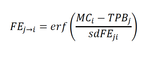
The standard deviations used in the equations above are depicted in Eq.21 and Eq.22.

D.3 Market share dynamics

Based on these consumer preferences (both EoL and premature), market share changes can be estimated. While market share changes are informed by preferences, they are not the only deciding factor. The uptake of new technologies is constrained by the production capacity of such technologies. Furthermore, new technologies may only come in when existing technologies need to be replaced, either at the end-of-lifetime or prematurely. The market share dynamics should also portray the fact that (especially) consumer choices are influenced by behavioural patterns, besides the economic considerations (Grubb, Hourcade and Neuhoff 2014, Knobloch and Mercure 2016). One part of this comes through in the standard deviations associated with preferences, and another part comes through by taking into account the existing stock of each technology.

To estimate market share changes an adapted version of the Lotka-Volterra equation will be used. The Lotka-Volterra equation is more commonly known as the "predator-prey" equation in the field of ecology, where it originally stems from (Volterra 1926, Lotka 1920).

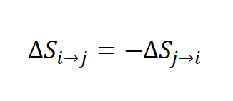
For market shares to move from technology to technology , it is deemed to be proportional to: pre-existing market shares of both technologies; how fast technology can be built; by what rate technology is decommissioned; and the preference for over . This is shown in Eq.23. The opposite is also true, see Eq.24.

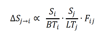
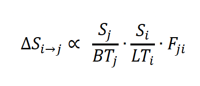
Where: S is the market share of a technology; BT is the build-time; LT is the lifetime; and F is the preference.

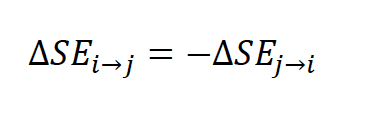
By combing both equations above, the net market share change from technology to (which may be negative) can be estimated. This is expressed in Eq.25 and Eq.26.

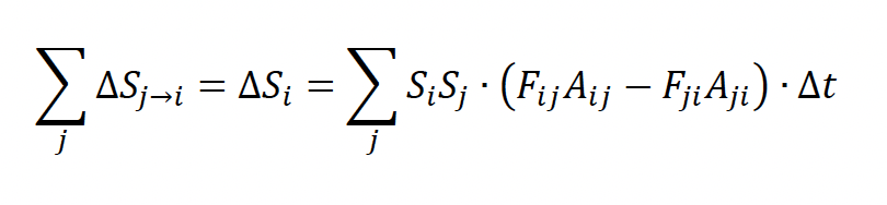
Where: A_ij is the substitution rate by which technology i can substitute technology j, given by Eq.27.

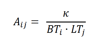
Where: κ is a time constant.

Similarly, for estimating premature market share changes depend on the MC and TPB driven consumer preferences (FE), the pre-existing market shares and the scrappage rate (SR). This is depicted in Eq.28 and Eq.29.

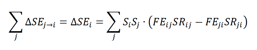
Where: SR_ij is the scrappage rate by which technology i can prematurely substitute technology j and is given by Eq.30. It is the inverse of the pay-back period minus the EoL replacement rate to make sure to exclude EoL replacements from the premature replacements dynamics.

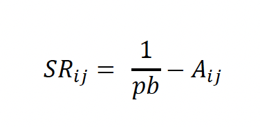
Where: pb is the pay-back period.

D.4 Simulating the effect of policies

Policies may change the rate of technology uptake through a variety of ways. In this analysis, subsidies are used to amplify the attractiveness of renewable heating technologies. They do so by lowering the investment cost component which lowers the LCOH and MC and therefore amplify the preferences to substitute towards the subsidised technologies.

Phase-out regulations on high carbon heating technologies will change the investor preferences. If a full phase-out is simulated, then the preferences for substituting towards these technologies is set to zero.

Biomethane blending will lower the emission intensity of gas boilers as a proportion of the gas burned displaces fossil fuel gas. It is assumed that the production of biomethane takes up as much carbon dioxide as is released during combustion.

Government procurement or kick-start programs are modelled as exogenous market share changes which may affect market shares at any given time in combination with EoL and premature market share changes.

Technological limitations & assumptions

Not all heating technologies are suitable for every building. For example, residents of flats face a space constraint and therefore it is unlikely that technologies such as solar thermal or individual heat pumps can be installed to supply those dwellings with renewable heat. To prevent the model from simulating an erroneous uptake of particular technologies for particular building types, constraints have been put in place. These constraints apply to all scenarios.

In this analysis it was further assumed that communal heating does not increase in market shares as it is not a consumer decision but rather a centralised decision. Gas grids were also assumed not to be expanded anymore. This was reflected in the model by setting maximum market shares for gas boilers in each local authority and in each building domain (non-domestic, domestic flats, and domestic houses).

To mimic learning-by-doing by global uptake of heating technologies, an exogenous decrease of investment costs was implemented. This decrease was informed by a baseline scenario of the global E3ME-FTT model, operated by Cambridge Econometrics.