Development of a combined marine and terrestrial biodiversity indicator: research

7. Stakeholder consultation and decisions made

113. This chapter describes the process of decision-making by the project team, the Scottish Government Research Advisory Group, and through consultation with a range of stakeholders. We highlight the key issues raised and decisions made through this process.

114. Consultation with a broad stakeholder community was conducted through three workshops and accompanying email correspondence (e.g. with experts unable to attend), through three meetings with a Scottish government-convened Research Advisory Group, and with the Scottish Biodiversity Strategy Science Support Group through attendance at one meeting and the circulation of a short document for consultation (Appendix 2).

7.1 Stakeholder workshops

115. Workshop 1, 23^rd April 2019, City of Edinburgh Methodist Church: engagement with stakeholders in terrestrial and freshwater biodiversity data, with a focus on conservation professionals involved in biodiversity monitoring and the use of biodiversity data for conservation decision-making. A list of attendees is given in Appendix 2.

116. Main topics discussed: an introduction to the project and its aims; existing biodiversity indicators; reviewing biodiversity data and its suitability; data flows and how producing an indicator might work; issues and identifying priorities for improving data availability.

117. Conclusions:

• A general support for the project, and Scottish Government's intention of producing a new NPF indicator. Partners willing to provide data for inclusion.
• A number of datasets not identified in our original review were suggested for consideration (e.g. SEPA dataset on freshwater invertebrates, biting midge monitoring, Rivers Trust fish data, tipulid flies, estuarine fish) (although none were included in the proposed indicator following subsequent investigation).
• Agreement with the project team's focus on an indicator based on the average trend in species' status.
• Consensus that the recommended indicator should not be regarded as static, but as a starting point with the aim of improvement in subsequent iterations (e.g. through the inclusion of more trends to make the indicator more representative).
• A clear call for actions that will support the biodiversity monitoring in Scotland (and in turn support the future improvement of the indicator). A wide range of points were raised in this regard, including the following: supporting and developing the biological recording community in Scotland, particularly by developing new recorders and prioritising effort at particular gaps; securing long-term funding for monitoring and recording schemes; develop new systematic monitoring schemes for key taxonomic groups; strong support for the implementation of the recommendations of the Scottish Biodiversity Information Forum (SBIF) review (Wilson et al. 2018);
• Concern that the indicator will not function in a 'useful' way – that the requirement to have a single headline metric will mean it will not be responsive, and indicative of changes in biodiversity in a way that will stimulate responses. It was felt that as well as the best possible indicator design, strong communication of how the indicator was created, and how changes (or lack of changes) in the indicator should be interpreted were essential.
• As a consequence of the point above, there was a clear and strong support for the publication of disaggregated indices at a level that would enable better understanding of changes in Scottish biodiversity than the headline indicator alone. A number of options for this disaggregation – e.g. by taxa, habitat, region – were discussed, as well as possibilities for the publication of such indicators.

118. Workshop 2, 24^th April 2019, RSPB Scotland Headquarters, Edinburgh, engagement with stakeholders in marine biodiversity data. A list of attendees is given in Appendix 2. The main topics discussed included: an introduction to the project and its aims; suitable marine biodiversity data sources for use in an indicator; spatial and temporal extent; relationship with existing marine indicators; indicator construction.

119. Conclusions:

• Agreed that the marine element of the indicator should be regarding as reporting on biodiversity within the Exclusive Economic Zone (EEZ), so a range of up to 200 nautical miles.
• A range of potential data sources were discussed, the principal amongst them being Seasearch; MarClim (covering a range of intertidal taxa), data on seabirds and cetaceans collected at sea and collated through the MERP project; OBIS (offshore benthos), Continuous Plankton Recorder and Marine Scotland plankton sampling, and fisheries data.
• However, it was recognised that most of these have not yet produced robust species trends suitable for use in an indicator, and the work required to do so was beyond the resources of this project.
• The issue of trends being influenced by factors outside of Scottish waters was discussed, but it was acknowledged that little could be done about this, and it was true for all biodiversity to an extent.
• As with terrestrial biodiversity, felt important to use the longest timeline possible to illustrate past biodiversity change.
• Concerns expressed whether trends derived from fish abundance would reflect ecological change, or could perform perversely, for example as overfishing results in an abundance of small individuals.
• Content to use trends in both abundance and occupancy (if and when the latter become available).
• The issue of weighting elements of the indicator to address biases in data availability was discussed, but nothing concluded.
• As with the terrestrial discussion, there was a clear interest in disaggregation of a headline metric for example by habitat (substrate), functional group or region.

120. Workshop 3, 17^th July 2019, City of Edinburgh Methodist Church: engagement with Scottish Government stakeholders, with additional input from conservation, monitoring and research stakeholders. A list of attendees is given in Appendix 2. The main topics discussed included: available biodiversity data; options for producing an indicator, including draft versions; understanding and communicating the indicator; requirements to enable future revisions, and potential for improvements; conclusions and next steps.

121. Conclusions

• Valuable input was received on issues regarding data proposed for use in the indicator, covering a wide range of points: need to understand risks around data supply and hence potential issues with future updates; potential future evolution of the indicator as new data becomes available.
• Datasets for future inclusion were discussed. These include a large number of freshwater biodiversity records available from SEPA. As yet these data have not been added to the BRC database, so are not currently available for the Bayesian occupancy analyses contributing species' trends to the draft combined indicator, but the intention it that this will happen so future analyses will benefit from these records, leading to more robust trends for species included already, and very likely to trends being derived for a larger suite of freshwater species.
• As with marine workshop, there was discussion over whether using fish abundance was appropriate as a measure of marine health.
• There was considerable discussion on start date of the indicator, with general support for it starting as early as possible. 1994 was identified as potentially the most suitable date.
• On balance, attendees agreed with the intent of combining both abundance and occupancy, although not all agreed.
• The use of weighting to address biases in data availability was discussed; although there appeared to be some support for this as a concept, there was no clear advice or opinion on how this should be done in practice.
• Concerns were expressed by a number of attendees over the requirement of producing a single line indicator, with some frank opinions of the limited value of this, and potential problems it might cause for policy use, funding efforts, communication – in effect being an impediment to successful nature conservation in Scotland.
• As in all other consultation conducted as part of this project, there was considerable discussion on and strong support for the need for simultaneous and linked publication of disaggregated indicators (possibly by SNH) to improve the value of the headline indicator. There was discussion over the various forms of this disaggregation – taxon, trend currency, realm, habitat, functional group, geography, drivers of change – whilst acknowledgement that not all of these would be possible.

7.2 Research Advisory Group

122. Meetings of a Scottish Government-convened Research Advisory Group (RAG) were held on 14^th Jan and 15^th May 2019. RAG members were updated on project progress and provided guidance on project requirements and particular issues. Key input was received on set of questions raised in advance of the meeting on 15^th May, via a short note circulated to the RAG electronically. This is given in Appendix 2, along with notes on the decisions made by the RAG. We summarise these here:

• The indicator should conform to NPF indicator template, being a single index presented without any estimate of error. There was, however, strong support for the separate publication of a suitable range of disaggregated indices to provide contextual supporting material.
• The balance of opinion was in favour of a broad composite indicator created from species' trend data. It was felt preferable that this be capable of being updated annually, with a time lag in reporting of no more than three years. A long timeline (i.e. as early a start date as possible) was supported.
• The RAG agreed that the indicator might be subject to future development to address shortcomings (e.g. poor representativity of some taxa or ecosystems) which might result in retrospective changes to the indicator.
• There was considerable discussion on the use of trends of species' abundance, and trends of species' distribution; the relative merits of each, whether one should be preferred over the other, or whether the two should be combined in a single metric.
• Other discussions centred on issues around marine data.

7.3 Scottish Biodiversity Strategy Science Support Group (SBS SSG)

123. One of the project team (ME) attended a meeting of the SBS SSG in early 2019 to outline the project requirements and the plan for the work to be conducted. Due to the lack of a suitably-timed meeting, it was not possible to discuss the final recommendations arising from the project at a further SSG meeting, so a short note outlining the proposed indicator was circulated in mid-September. This included decisions made through the process of consultation outlined above, but also those final decisions made by the project team and outlined in section 7.4 below.

124. Responses were received from five members of the SSG. All were broadly supportive of the recommendations of the project team, including the key decisions highlighted within the note. The common denominator in the feedback received was strong support for recommendations that disaggregated indicators should be produced to support interpretation and understanding of patterns of change shown by the headline indicator.

7.4 Further decisions made by the project team

125. The consultation described above guided the project team through many most of the decisions required to identify a suitable indicator. However, there were a number of remaining decisions to be made.

7.4.1 Data

Rules for the inclusion of species' trends

126. Trends for individual species have only been considered for inclusion in the indicator if considered to be sufficiently robust. For abundance trends, we have relied on assessments provided by those responsible for overseeing schemes. For example, we have only incorporated trends for breeding birds from the BTO/JNCC/RSPB UK Breeding Bird Survey if considered sufficiently robust for publication (i.e. species that have been recorded from a minimum annual average of 30 survey squares within Scotland over 1994-2018 course of the survey). Similar assessments have been applied to other bird data sources and those for mammals, moths, butterflies, marine mammals and fish.

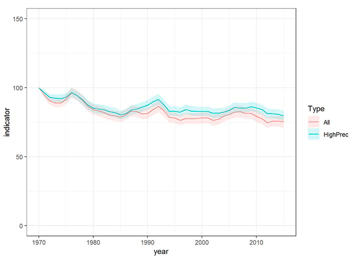
127. For the broad sweep of species for which we derived trends in occupancy from biological records through the application of Bayesian modelling techniques, a similar threshold approach was applied. We first explored a threshold based on the number of records (i.e. the sample size per species). Lower sample size thresholds may result in individual species' trends that were less robust being incorporated within the indicator. Higher thresholds will exclude such species, as a consequence reducing the number of species' trends which can be incorporated within the indicator. We found that below threshold of 50 records the models did not produce sufficiently robust results. It is not apparent that a higher threshold can be justified a priori, so we looked instead at the precision of the trend estimates that emerged from the occupancy models. Whilst species with larger sample sizes tended to have more precise trend estimates, there are many species that buck this trend: on the one hand rare species with few records and precise trends, and widespread species with many records and imprecise trends. However, the distribution of precision across species is clearly bimodal (Pocock et al., draft report to JNCC), implying a clear separation between "precise" and "imprecise" trends. One option would be to take the midpoint between these modes as a precision threshold, but in practice it makes a negligible difference to the resulting indicator line, particularly the trend since 1994 (Figure 1). In other words, the "imprecise" trends merely add noise, not bias. In the absence of an objective threshold, we therefore suggest using the full set of 1763 occupancy model outputs.

128. For a few species of birds and moths, trends were available from more than one source. In such cases we have identified a hierarchy for identifying the most suitable trend for incorporation. We have given precedence to assessments of change in abundance, as this is thought to be the most sensitive measure. In the case of multiple abundance trends being available for a species, we selected the trend from the dataset believed to be the most robust, based on the survey method subject to the fewest known biases, and maximising the sample size and time period covered. For example, for bird species for which trends in both breeding and wintering abundance were available, we gave precedence to the breeding population trend.

Marine Groundfish (demersal fish) data

129. For the marine data, there exist different versions of the ICES bottom trawl datasets. ICES serve these data directly via their DATRAS data portal in close to real time, and they provide web services allowing programmatic access. We developed a workflow in the statistical computing environment R to access and process the data directly, adding specific functionality (e.g. subsetting to Scottish waters, deriving species-level abundance trends) on top of open source tools developed within ICES. The key advantage is that this entire workflow can be replicated to access updates to the DATRAS database, so that the resulting index can be updated to incorporate new data from these ongoing surveys.

130. However, there are persistent concerns about the level of quality control conducted on ICES data, particularly in earlier years. This led the Scottish Government to invest in a high degree of quality control of ICES trawl surveys in order to support the OSPAR interim assessment in 2017. These data products are provided by Marine Scotland, and described in full here: Scottish Marine and Freshwater Science Reports. Again, we developed a workflow in R to process these data, sub-setting to the Scottish EEZs and deriving abundance trends at the species level. These trends are likely to be more robust than those derived directly from the ICES data, however they do not run past 2017 and additional resource would need to be committed year on year to perform equivalent quality control to all new ICES trawl survey, and publish these as new data products, or as revisions to the existing products. In addition, although these data products are openly available to download (which was our approach), programmatic access in R is not yet possible and so even if the data were updated, additional revision of code would be required in order to update the abundance trends.

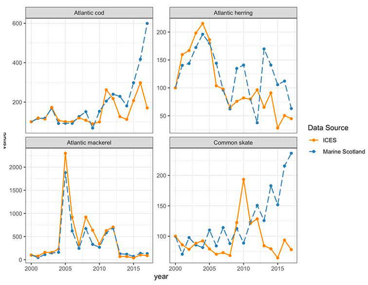
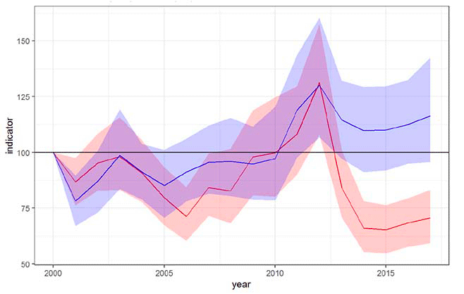
131. One common approach to this kind of problem is to use the period of overlap between time series to derive correlations which can then be used as a 'correction factor' for years in which only one data source is available. That is complicated in this case, however, because different units of abundance are used (the Marine Scotland data products use individuals per unit area, whereas ICES use individuals per unit time). It would be a substantial research exercise to work out how best to combine these two data sources, and is beyond the scope of our project. To better inform the choice between these two sources of trawl survey data, we did, however, compare both species-level abundance trends and the overall aggregated trend derived from both sources. We ran this comparison from the year 2000 on the assumption that quality control issues would be a lesser issue in newer ICES data, as processes have become better standardised. Although trends are similar for many species (Figure 2), there are also some substantial divergences, and the overall trends diverge substantially around 2012 (Figure 3).

132. It is our considered view that the advantages inherent in accessing ICES data directly from DATRAS – namely, a straightforward, repeatable programmatic workflow which can be updated year on year with minimal additional resource – makes this the best choice for the current purposes. This is not to ignore the data quality issues addressed by the Marine Scotland products, but the general concordance in species-level trends between the two data sources (Figure 2) reassure us that the advantages of an easy-to-update index that does not require additional annual resource outweigh these concerns.

7.4.2 Indicator start and end date

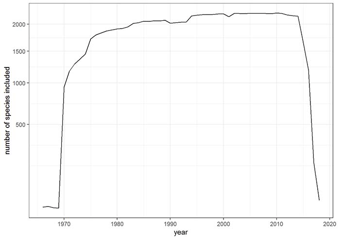
133. Many of the stakeholders who partook in the consultation exercises described above expressed a wish for the indicator to extend back in time as far as possible, in order to provide context to current day changes. This desire has to be balanced against changes in data availability through time, and variation in the robustness of the indicator, and consistency of what change the indicator is measuring. Figure 4 shows how, using the data for 2,073 species as described above, the number of species contributing to the indicator increases through time. Trends in wintering waterbirds are available from 1967 onwards, trends in occupancy for many species are available from 1970 onwards (hence the massive jump at this date). Smaller but significant increases in species sample size arise with the addition of taxon-specific monitoring schemes, for example the Rothamsted Insect Survey (moth trends) in 1975, the Seabird Monitoring Programme in 1986, and the UK Breeding Bird Survey in 1994.

134. We recommend 1994 as the start date for the indicator. Although further species trends are incorporated in the indicator in subsequent years (e.g. five species of bats and four species of terrestrial mammals from 1998 onwards), such additions have an extremely minor impact on the indicator and so do not justify delaying the start date. Whilst an earlier start date would be possible – after all, the majority of the trends used in the indicator are available from 1970 onwards, the lack of data on vertebrates during this period means the indicator line would not be representative of biodiversity as a whole.

135. Similarly, the choice of the current end year also requires careful consideration, because of the time-lag in making data widely available. Setting it too early would make the indicator out-of-date; setting it too late would be unrepresentative of all biodiversity. The number of species with data drops off markedly after 2014 (Figure 4) and is very low indeed for the most recent years (29 species in 2018, 191 species in 2017). We believe that 2016 represents a reasonable compromise based on current data: there are 1003 species with data for this year, and all major taxonomic groups are represented.

7.4.3 Indicator creation

136. The consultation and decision-making outlined above left two significant decisions to be made, concerning how the species' trends identified for inclusion should be combined into an indicator. The first question concerned whether to use weighting (also referred to as 'stratification') to attempt to correct for biases in the availability on species' trends. The second is which technique should be employed to create the indicator, and how the uncertainty should be represented.

137. We chose to weight all 2,073 species equally, regardless of taxonomic group and whether the data represent trends in occupancy or abundance. This choice reflects the fact that any choice of weighting is necessarily subjective, and we lack a clear rationale for favouring any one of the available choices. One could weight species by the degree to which different taxonomic groups are represented (as in the WWF Living Planet Index), but this requires some choice about how to delimit the taxonomic groups. For example, should "birds" be considered a taxonomic group, or should birds, mammals and fish be grouped together as 'vertebrates'? If weighting is employed, there also remains a decision about whether the purpose is to introduce equality between groups (e.g. giving equal weighting to each taxonomic group), or to reflect the relative diversity of such groups (e.g. giving increased weighting to invertebrates to correct for the lower proportion of all invertebrate species included in the indicator). Our choice of an unweighted indicator does not represent a strong preference for this approach, but rather a lack of preference for any alternative. We suspect the difficulties in identifying the most appropriate use of weighting to address biases in data availability underpins the widespread and continued use of unweighted indicators e.g. in other countries.

138. We compared two methods for indicator creation, both of which seek to estimate the geometric mean of the species index values. The first approach is a simple geometric mean across species, adjusted to account for missing values (species:year combinations with no data). Confidence intervals are calculated from a bootstrapping procedure in which the indicator is recalculated 1000 times. In each of these 'bootstraps', species data are sampled with replacement to create a dataset equal in size to the original (2073 species) but differing in composition (some species absent, some replicated several times). This is the method used for the UK Priority Species indicator, and for the State of Nature reports (methods described in Burns et al. 2018). The resulting index has substantial confidence limits around it, and considerable year-to-year variation (blue line in Figure 5).

139. The second approach is a new hierarchical modelling method for calculating multi-species indicators within a state-space formulation developed by CEH (Freeman et al. 2020). Model-fitting is straightforward in either Bayesian or classical inference implementations, the latter following from efficient hidden Markov modelling. As the indicator presented in this report was calculated using the Bayesian approach, hereafter we refer to it as the 'Bayesian' indicator. The key features of this method are 1) species index values are assumed to be imperfect, and 2) the indicator is smoothed in-situ rather than post-hoc. The resulting line varies less from year-to-year (compared with the geometric mean) and is substantially more precise (narrower ribbon of uncertainty on Figure 5). A further difference with this approach from the 'conventional' geometric mean indicator is that the imputation of missing values is informed by between-year change in species for which data is available, which means that for the terminal year the indicator may be more appropriate than that obtained using the geometric mean method, which assumes no change in index values for missing species.

140. We believe the second, new, approach to be most suitable for use for the new combined indicator; it is robust, precise, adaptable to different data types and can cope with the issues often presented by biological monitoring data, such as varying start dates of datasets and missing values. This approach is likely to be adopted for the production of biodiversity indicators elsewhere including some of those produced for official indicator suites for the UK and England. As Figure 5 shows, the two methods provide similar results.

7.5 Summary

141. In this chapter we have outlined the consultation process undertaken as part of this project, with Scottish Government and a wide range of other stakeholders in biodiversity policy, research and conservation.

142. The consultation process clarified the requirements of Scottish Government for an indicator to be included within the NPF indicator suite, so consisting of a line showing variation in a single measure over time.

143. Using the input from stakeholders received through this consultation we were able to make the key decisions on data to be used in a combined indicator, the treatment of this data, and concerning issues around the construction of the indicator itself such as start and end dates, the combination of data measuring both trends in abundance and occupancy, whether to use weighting to address biases in data availability, and the statistical method used to generate the indicator.

144. Our recommended approach for a combined biodiversity indicator for Scotland is given in Chapter 8.