Bird stomach contents analysis - final report: Goosander and Cormorant diet on four Scottish rivers 2019 to 2020

2. Methods

Stomach contents analysis

Full details of the stomach contents analysis and diet assessment methodology used in the present study are given in Appendix 1 and published sources (Marquiss et al. 1998 and references therein, Feltham 1990, Carss & Ekins 2002, Carss et al., 1997).

The sampling unit for stomach contents analysis is not the number of fish recorded in a stomach but the stomach itself. Sample size is important as it can affect the accuracy of diet assessments, with some fishes being 'missing' from smaller samples of birds. In Scotland (where the fish community comprises relatively few species) it has been concluded that 'adequate' estimates of Goosander and Cormorant diet (i.e. relative proportions of different prey species by mass) were possible from samples of 12-15 stomachs containing food (Marquiss & Carss, 1997). An important consideration for the present work was thus acknowledging that a sample of fewer than 12 stomachs with food is likely to be too small to ensure it is representative of general diet. The full process of carcase dissection and stomach contents analysis is described and illustrated in Carss et al. (2012) but is described briefly here.

After taking biometric measurements (Appendix 2), the body cavity of the bird was opened, following the digestive tract, down the length of the neck to the vent. Any whole, intact, undigested fish were removed, identified and measured (length, mass) whilst all remaining partially-digested material were carefully flushed out into a storage jar. A saturated solution of biological washing powder was added for a few days in a warm oven in order to digest all the remaining flesh from partially-digested fish. Then the contents of each jar were sieved and thoroughly rinsed with cold water before being air dried on filter paper for 1–3 days. There is no evidence that exposure to biological washing powder damages bones nor that air drying leads to significant shrinkage over periods of at least a few months.

The resulting dried prey remains were examined under a low power binocular microscope and 'key' bones identified to species level. These key bones included the atlas vertebra (for Salmonids), paired pharyngeal teeth (Cyprinids) and pelvic bones (3-Spined Stickleback), and other vertebrae and lower jaws (dentaries). Key bones were counted (as left/right pairs if necessary) and measured - bone lengths being converted to estimated fish lengths using regression equations, and estimated fish lengths to estimated fish mass, also with appropriate regression equations. Extremely well-digested - and hence heavily eroded and damaged - bones were excluded from analysis at this stage. Any data obtained from whole, intact, undigested fish were included with those determined from the examination of key bones from partially-digested material.

Ultimately, the minimum numbers of each fish species were recorded for each stomach and a cumulative total produced for each sample of birds. At its simplest, general diet can be assessed as the presence/absence of different prey species and presented as frequency of occurrence (e.g. 'percentage frequency' - the proportion of stomachs containing a particular species). Estimated prey fish body masses were summed for conspecifics in each sample of stomachs. Finally, the contribution each species makes to the total mass was calculated and presented as relative frequency for a particular sample.

Importantly, the material examined during this stomach analysis process was 'fresh', having usually been consumed no more than hours before birds were sampled. Whilst Goosanders and Cormorants have different digestive tracts, both digest fish quickly and in distinct stages.

Cormorants regurgitate an oral pellet each day and these contain the hardest, indigestible parts from prey, covered in mucus produced from the stomach lining. Consequently, any stomach contents found in Cormorants can only have been consumed in the previous 24 hours. Goosanders do not produce oral pellets but instead have a muscular proventriculus, often containing grit and small pebbles which help to grind prey items, thus aiding digestion and reducing the residence time of stomach contents. For both birds species, careful examination of any visibly damaged and/or eroded (i.e. well-digested) key bones from stomachs, and the exclusion of these from analysis, further ensures that diet assessments are tightly associated with the date of sampling. It is thus highly likely that such dietary assessments are derived from the prey consumed by birds on the day of sampling or possibly the previous day, but seldom – if ever – any longer ago than that.

Following Marquiss et al. (1998), general diet as assessed from stomach contents is reported here for each prey species in terms of (i) numbers, (ii) estimated mass, and (iii) frequency (% by mass). In Section 4, these data are tabulated and a graphical comparison is made (by river stretch and/or time of year) with any available relevant historical (1990s) samples from Marquiss et al. (1998). In Section 5, the estimated length frequency distributions for Atlantic Salmon (Salmo salar) from both the 2019 smolt run and autumn-winter 2019/20 sampling periods are compared with relevant historical data and with each other. It should be noted that historical fish length frequency distribution data were never digitised and so the length frequency comparisons presented here are limited to those still available for individual fish as hard copy.

Additional fish identification and biometrics methods

In addition to the published sources for diet assessment cited above, the bone to fish length and length:mass equations of Hájková et al. (2003) were used here for Grayling, and those of Britton & Shepherd (2005) for Gudgeon and the largest Minnows. To estimate the mass of the single (fresh, intact) Grey Mullet, the length:mass equation for Salmon was used, as this is a species of similar body shape. Throughout the report, any Salmonid more than 30cm in length was arbitrarily categorised as being "large" to differentiate it from juvenile individuals. Such fish were identified as either adult Salmon or large Trout (either resident, or migratory 'Sea Trout') where possible, based on the pattern of teeth on the vomer – with Trout having a well-developed double row of teeth and Salmon a less developed single row. Where species identification was not possible, fish were recorded as 'large Salmonid'. The lengths of these large Salmonids were determined by averaging the length estimates derived from measurements of the atlas vertebra, lower jaw (dentary), and caudal vertebrae (cf. Carss & Brockie, 1994) and from direct measurements and comparison to the body proportions (i.e. tail to anterior edge of dorsal fin vs anterior edge of dorsal fin to snout) of the ingested fish and reference photographs of live Salmon. In one case, body length was estimated from the circumference of the caudal penduncle (Carss et al., 1990).

Statistical methods and a note on presentation

The estimated Salmon length frequencies for different samples of birds (Section 5) were compared using the Kolmogorov-Smirnov test, adapted for data sets following discrete or mixed distributions (Arnold & Emerson 2011, Dimitrova et al. 2020). This is a non-parametric statistical analysis with a null hypothesis stating that there is no difference between the two length frequency distributions. The test has no restrictions on sample size and so small sample sizes are acceptable (Siegel & Castellan 1988). The test was chosen because it is distribution-free, adapted for discretised data with repeated measurements, and is applicable to data with bi/multi-modal distributions. The test statistics was specified by:

D = supx | F1 (x) – F2 (x)|

where F1 (x) is the empirical distribution function of the data samples from one sampling period and F2 (x) is the empirical distribution function of a second data sample.

Reported p-values were estimated by Monte Carlo simulations with 10,000 replicates, and those were then compared to the exact p-values obtained using the Fast Fourier Transform method (FFT). The threshold of probability was taken to be 0.05 and p-values (exact KS-FFT method) are presented. Full details of the methodology are given in Arnold & Emerson (2011) and Dimitrova et al. (2020), respectively. Tests were performed using the ks.test function in R (dgof library) and the disc_ks_test function in R (KSgeneral library).

Salmon length frequency distributions are presented graphically in three ways in Section 5. First, histograms of estimated length frequency (% by number) for 10mm length categories are given. Many of these show that the Salmon have bimodal or skewed length distributions, hence the need for non-parametric statistical testing as detailed above. Second, boxplots are presented to show the distribution of the length data, its skewness and non-Normality. For comparative samples of estimated Salmon lengths, these boxplots give median values (the middle value of the dataset), the 25th and 75th percentiles (medians of the lower and upper halves of the dataset, respectively) and the minimum and maximum estimated length values within a distance equal to the interquartile range x 1.5. The dots show the points that are beyond this distance. Finally, plots of empirical Cumulative Distribution Functions (ecdf) are presented for the estimated Salmon length frequency comparisons. These are plots of the distribution functions associated with the empirical Salmon length measurements for different samples. Length differences between samples are apparent from ecdf plots but they also provide some summary statistics. For example, Figure 1 is an ecdf plot of the proportions (Y-axis) of Salmon lengths (X-axis) for three annual samples and shows the proportion of fish with estimated lengths of 60mm or less was 45% in 2019, 19% in 1995, and 8% in 1996.

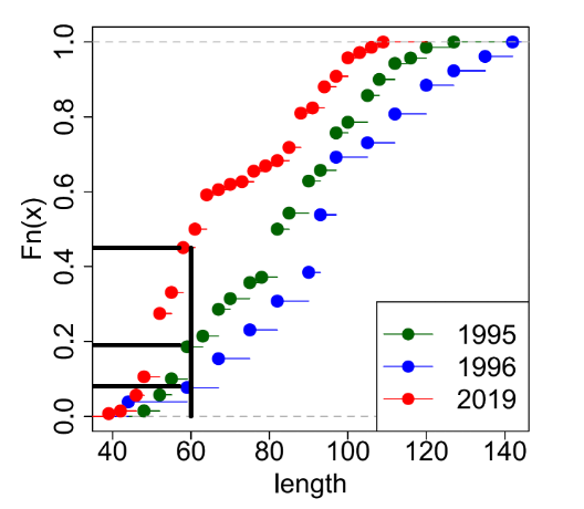
Statistically, this ecdf plot is the distribution function associated with the empirical measure of a sample set against a cumulative probability on the Y-axis that ranges from 0 (0%) to 1.0 (100%) and with Salmon lengths on the X-axis sorted (left to right) from shortest to longest. The ecdf is a step function represented by a series of dots with tails. Each dot represents a (sorted) fish length with a tail extending to the right until the next (sorted) length is reached whereby the distribution steps up to this next point. The cumulative distribution function value at any specified point of the measured variable is the fraction of observations of the measured variable that are less than or equal to the specified point.

The ecdf is an empirical (step) function, where 'empirical' means that it represents the observed values and the corresponding data percentiles. The step function increases by a percentage equal to 1/"Sample size" for each observation in the data set. As an example, the 2019 season (Figure 1) has 142 observations and the step function increases by 0.007 for each observation. Thus, the probability of fish with length of 46mm or below would be 0.007 multiplied by 8 observations, which is 0.056 (or 5.6%).

Statistical analysis for stomach contents samples

For a limited number of samples, it was possible to investigate statistically any differences in diet assessments using K-S tests and following the same procedure as described above but comparing the estimated mass of each fish species recorded in each stomach that contained food.

Such data were recorded for all stomachs examined in the present study, although comparisons were limited by the numbers of stomachs containing food in each 'paired' seasonal sample. On occasion, Marquiss et al. (1998) made dietary comparisons (their p. 38) or estimated species 'intake rates' per 100g of food (their p. 54) based on samples of at least five or ten stomachs with food, respectively. Given this, in order to be able to include data from late autumn 2019, samples with 11 or more stomachs with food were deemed 'valid' in the following statistical analysis. Historical data in the required form (i.e. mass of each prey species per stomach with food) were only available for a single previous sample (Tweed Goosanders, April 1992, N = 55 birds containing food). Consequently, statistical comparisons of general diet were made between samples of Tweed Goosanders in the smolt run period 2019, spring 1992, autumn 2019, and both early and late autumn 2019 separately.

Within each sample of stomachs containing food, the mass of each fish species recorded will either be zero or a positive value, with zero values counting towards the total sample size for statistical tests. Simulation studies to understand what sample size and what number of positive values within a sample might be appropriate was outwith the scope of the present study. Therefore, a threshold sample size of five stomachs was chosen subjectively (D. Sadykova, pers. comm.) in order to reduce the 'uncertainty' of diet estimates for samples where a particular fish species is only recorded in a small number of stomachs. Thus, to increase confidence in the interpretation of the statistical tests, any samples of stomachs with records of a particular prey fish in none, or only 1, 2, 3, or 4 of them, were excluded from analysis.

As before, K-S tests are reported as D-statistics and p-values (KS-FFT method), and data are presented as boxplots and ecdf plots. For each fish species within a sample of birds, plots were determined from all stomachs containing food, and so they include zero values whenever a particular fish species was absent from a stomach. For boxplots, median values were calculated for the full sample of stomachs (including zero values) and so show the median estimated mass (g) of a particular fish species in any particular sample of birds. Statistical comparisons of the general diet estimates between pairs of samples could not be made if all of the stomachs in either sample contained no records of a particular species.