Scottish Shelf Model. Part 6: Wider Domain and Sub-Domains Integration

5. Particle tracking model

5.1 Introduction

A particle tracking and connectivity methodology report (Wolf, 2015) has been prepared and reviewed by Alejandro Gallego (Marine Scotland Science) and Prof Christina Sommerville (Emeritus Professor of Aquatic Parasitology, Institute of Aquaculture, University of Stirling). This full report is attached as Appendix A while some extracts are included here. The initial statement of the problem is to deliver "Connectivity indices (which may be defined as the degree of dynamic interactions between geographically separated populations via the movement of individuals), such as transition probability matrices between (finfish aquaculture) Farm Management Areas ( FMA)." These FMAs are on the west coast of mainland Scotland, the Western Isles, Orkney and Shetland; 86 FMA polygons are identified, from which particles are released and tracked and their capture by the original or other FMAs is calculated.

The report reviews the background to this study in terms of the dispersal of sea lice, referring to the life cycle of the sea louse Lepeophtheirus Salmonis (referred to as L. Salmonis, also known as Leps) which is the main species causing concern in the aquaculture industry, as well as the behaviour of 2 other disease vectors: Infectious Salmon Anaemia Virus ( ISAV), a representative short-persistence pathogen and Infectious Pancreatic Necrosis Virus ( IPNV), a representative long-persistence pathogen. Some previous particle tracking studies are reviewed.

Based on laboratory experiments, the optimum temperature for L. Salmonis larvae is 10°C and the optimum salinity is 33-35 psu. The larvae are infectious when they are in the copepodid stage (approximately the last ⅔ of the pelagic larval duration, PLD). At lower salinities copepodids do not thrive (< 25 psu). Copepodids are thought to maintain their position just below the halocline when surface water is less saline than 29 psu. Otherwise they are in the surface waters (they control this by buoyancy and vertical swimming behaviour). Representative particles are therefore released in the surface layer and "target" FMAs reached within the infectious part of the PLD are scored.

ISAV has a pelagic duration of about 3 days and IPNV has a pelagic duration of about 35 days during autumn to spring and 17 days in summer. These disease vectors are assumed to be well-mixed through the water column and passive, so whole water column releases and passive vertical and horizontal drift (including diffusion) are used. All "target" FMAs reached within the pelagic duration period are scored.

The method adopted is to use the offline particle tracking module available in FVCOM (described in section 5.2). Some code fixes were necessary in order to get the horizontal and vertical diffusion parts of the code to work. The particle tracking is run in post-processing mode, using the Climatology output from the combined Stage 1 Shelf Model and Stage 2 models results ( sections 3 and 4), using the methodology described in sections 5.3, which utilises hourly current fields, forced by climatological forcing over a standard tidal year.

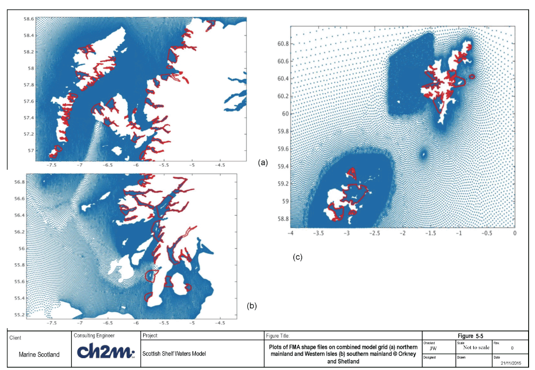
The FMAs are shown in Figure 5-1 to 5-4. They are represented by 89 shape files within the model grid ( Figure 5-5). The nomenclature used in Figs. 5-2 - 5-4 is used hereafter i.e. S1-S11 (Shetland, including S8a and S8b), O1-O4 (Orkney), M1-M49 (Mainland) and W1-W22 (Western Isles). Of these 89 areas, one represents a tiny extension of M13 and another is a westward extension of W14. Most of the FMAs are well-resolved in the combined shelf model mesh, however there are some that do not include any nodes of the model (M12, inner Loch Broom and M43, inner Loch Striven) and some that are only partially resolved ( e.g. S10 and M13). The FMAs numbered M11, M12 and M13 have therefore been combined within a boundary further out into the estuary and called LB (Loch Broom), see Fig. 5-6a. The inner FMA in Loch Striven (M43) has been extended south in order to enclose some model nodes ( Fig. 5-6b). The resulting 86 polygons have been used to define the areas of sources and sinks for particle tracking.

A large number of particles are released within the 86 Farm Management Areas ( FMAs) in Scottish Waters. The experimental design is described further in section 5.3. Example results of the particle tracking are shown in section 5.4

The Connectivity matrices have been calculated from these results, taking into account the length of time for which sea lice larvae and viruses can survive at various temperatures in the sea. This is presented in section 6.

5.2 Particle Tracking in FVCOM

5.2.1 Theory

From the FVCOM manual (Chen et al., 2013) the Lagrangian particle tracking module consists of solving a nonlinear system of ordinary differential equations (ODE) as follows

(5.1)

where x is the particle position at a time t, d x/ dt is the rate of change of the particle position in time and v( x, t) is the 3-dimensional velocity field generated by the model. This equation can be solved using any method suitable for solving coupled sets of nonlinear ODE's such as the explicit Runge-Kutta (ERK) multi-step methods which are derived from solving the discrete integral:

(5.2)

Assume that x _n= x(t _n) is the position of a particle at time t=t _n , then the new position x _n+1= x(t _n+1) of this particle at time t = t _n+1 (= t _n +Δt) can be determined by the 4th order 4-stage ERK method where Δt is the time step. The dependence of the velocity field on time has been eliminated since the velocity field is considered stationary during the tracking time interval of Δt. It is important to understand that in a multidimensional system, the local functional derivative of v must be evaluated at the correct sub-stage point x in (x, y, z) space. On a 2-dimensional ( x,y) plane, for example, a particle can be tracked by solving the x and y velocity equations given as

(5.3)

Many users have added a random walk-type process into this 3-D Lagrangian tracking code to simulate sub-grid-scale turbulent variability in the velocity field. In FVCOM version 2.5, only the advection tracking program was included as described above, however version 3.1.6 (as used here) includes an optional random walk, R (uniformly distributed within the domain [-1,1]), where the horizontal diffusivity D _h is specified as a constant and the vertical diffusivity D _v is provided from the circulation model.

(5.4)

Some smoothing of the diffusivity may be required in the vertical (Brickman and Smith, 2002). A key property of a correct Lagrangian Stochastic Model is that it maintains an initially uniform concentration of particles uniform for all time. This is called maintaining the well-mixed condition (WMC). If the result does not conform to WMC this may be due to inadequate resolution of the hydrodynamic model. Ideally one should conduct statistical tests to ensure that the number of particles is sufficient for the investigation (Brickman and Smith, 2002).

The in-line particle tracking program can be run on both single and multi-processor computers. However, in the MPI parallel system, tracking many particles simultaneously with the model run on a multi-processor computer can significantly slow down computational efficiency, since particles moving from one sub-domain to another require additional information passing. Multiple runs of the particle tracking would also require re-running the hydrodynamic model. For this reason, it is suggested that users use the offline version of the particle tracking code.

5.2.2 Offline particle tracking code

The offline code is provided in the FVCOM package. This is not parallelised and runs on a single processor only. For large numbers of particles (O(100,000)) the calculations may be run on multiple processors by dividing the particles between processors, to speed up processing. Multiple runs can be carried out in parallel as long as the particles are from different spatial locations (multiple particles from one point may produce duplicate runs due to the nature of the random number generator).

Note that the supplied version of the offline particle tracking code had some software errors which have now been fixed. This code includes no biological behaviour, but particles can be released at different vertical levels and there are options for inclusion of a random walk diffusion term in the horizontal and vertical, as well as 3-dimensional advection. There is an option for a fixed level or a sigma-coordinate level for the release points.

The modules of the offline package are shown in Table 5-1. The main code is in offlag.f90, which includes the main program PARTICLE_TRAJ which in turn calls subroutines in offlag.f90, alloc_vars.f90, data_run.f90, ncdio.f90 and triangle_grid_edge.f90. The other modules set array sizes, initialise arrays and provide certain utility subroutines and functions.

Table 5-1: Modules of Lagrangian off-line particle tracking program

Module	Purpose
alloc_vars.f90	Allocates and initialises most arrays
data_run.f90	Inputs parameters which control the model run
mod_inp.f90	Decompose input line into variable name and variable value(s)
mod_ncd.f90	NetCDF utilities
mod_prec.f90	Defines floating point precision using kind
mod_var.f90	Sets global limits and array sizing parameters
ncdio.f90	NetCDF I/O: input time and output surface elevation and bottom depth
offlag.f90	Lagrangian particle tracking off-line program
triangle_grid_edge.f90	Define the non-overlapped, unstructured triangular meshes used for flux computations
util.f90	Utilities, from Numerical Recipes

The important parts of the code deal with particle advection, then optional dispersion using a random walk method. The method of vertical diffusion is given in Visser (1997) and Ross and Sharples (2004).

The code as supplied worked for advection only and for Cartesian coordinates but not for lat/lon coordinates. The start-up time is quite long (~2 hours for the large combined model grid). A modified code which shortened this set-up time for subsequent runs, by saving metrics calculated within triangle_grid_edge.f90 was provided (Pierre Cazenave, pers. comm.), however there was a bug in this code which has now been fixed. The code also did not work for horizontal and vertical dispersion, which is calculated using a random walk. The horizontal random walk had some errors, with some variable declarations needing to be corrected. Additionally, there was a problem with the vertical random walk: there was an error in the dimension of the vertical diffusivity, which is read in at nodes but has to be interpolated to elements.

5.3 Particle Tracking in SSM

The particle release points were generated by generating a uniform 2kmx2km mesh extending over the whole model grid then selecting those points which lay within the FMAs. This produced at least 1 particle release point in each FMA, except for 3 locations where a particle release point had to be generated manually. The final selection was 977 release points with between 1 and 100 particle release points per FMA ( Figure 5-7).

Multiple particles were released at each location, using a random walk to model the diffusion, checking that the result was not sensitive to the number of particles. 100 particles per release point seemed satisfactory. A limited number of particles were used due to computational constraints. The number of particles required is discussed by Brickman et al. in North et al., (2009) which also refers to Brickman and Smith (2002). In typical releases they tested 100-2000 particles, to ensure that the final result is not sensitive to the number of particles.

'Sea lice' particles are constrained to stay in the surface layer. For this it was found best to use the fixed depth option, with the initial depth below the surface as 3m and only horizontal diffusion. The particles do move in the vertical by advection, to some extent, but most particles stay within the surface layer (see Figure 5-8).

'Virus' particles were released at surface, mid-depth and bottom in the water column, using 50 particles at each level, which was a compromise from the ideal (100 particles at each of 10 levels) to avoid excessively long run times of the particle tracking code.

The particles were tracked for appropriate PLD periods for each season (see Table 5-2).

Table 5-2: Particle tracking runs

Biology	Season	Start date	Duration	Scoring	Number of particles (depth)	Physics
Sea-lice larvae	Spring	1 April	15 days	Hours 121-360	977 x 100 (3m)	Advection plus horizontal diffusion
"	Summer	1 July	10 days	Hours 81-240	977 x 100 (3m)	Advection plus horizontal diffusion
"	Autumn	1 October	15 days	Hours 121-360	977 x 100 (3m)	Advection plus horizontal diffusion
"	Winter	1 January	18 days	Hours 145-432	977 x 100 (3m)	Advection plus horizontal diffusion
Viruses ISAV + IPNV	Spring	1 April	35 days	All (1 st 3 days for ISAV)	977 x 150 (S, M, B)	Advection plus horizontal and vertical diffusion
"	Summer	1 July	17 days	All (1 st 3 days for ISAV)	977 x 150 (S, M, B)	Advection plus horizontal and vertical diffusion
"	Autumn	1 October	35 days	All (1 st 3 days for ISAV)	977 x 150 (S, M, B)	Advection plus horizontal and vertical diffusion
"	Winter	1 January	35 days	All (1 st 3 days for ISAV)	977 x 150 (S, M, B)	Advection plus horizontal and vertical diffusion

5.4 Results

The separation matrix for the 86 FMAs has been computed, taking a simple direct separation using plane geometry. The maximum separation between FMAs is 662 km, between the southernmost FMA on the mainland and the north of Shetland. From the climatology run the residual currents near the shelf edge are directed towards the NE and have a maximum velocity of 25cm/s, generally much smaller residual currents will be present nearshore, where the FMAs are located. At 25cm/s a distance of 324km could be covered in 15 days, however much smaller distances are more likely.

Figure 5-9 shows particle tracks for the January 35-day virus runs where the particles are released at surface, mid-depth and bottom. Each panel represents a sub-division of all the particles between 10 processors (as discussed in section 5.2.2). The first 9 processors have been used to each calculate 15,000 particle tracks; 150 particles released at 100 different release locations for each case. The 10 ^th processor tracked the remaining released particles (making a total of 146,550 particles). A final run was carried out for 3 release points (450 particles) which were not moving within the grid. The surface releases are shown in red, mid-depth are green and bottom are black. The tracks for particles released at different levels do not differ substantially, apart from the random walk component, because the particles move freely through the water column, unlike the sea lice larvae which are constrained to stay in the surface layer.