Scottish Shelf Model. Part 6: Wider Domain and Sub-Domains Integration

3. Integration of model results from shelf and local models

3.1 Introduction

As outlined in Section 2, a number of methods were considered for the integration of the shelf and local models. The selected method is described in Section 2.2.5 (Method 5). A new mesh is created incorporating the shelf and local model meshes and the results from the shelf and local models are interpolated onto the new mesh to create the integrated results file. This integrated file is required as an input file for the particle tracking model. Daily hydrodynamic model result files are required for the particle tracking model, therefore the process was repeated for each day of the year. Results for the PFOW and WLLS models are available for the full year. However the results for ECLH and SMB models are only available May through to October. Therefore it was necessary to create two different integrated meshes, one including all the local model meshes ( Figure 3-1 to 3-2) and one including only the PFOW and WLLS model meshes ( Figure 3-3 to 3-4). A full description of this method is outlined here.

3.2 Integrated model mesh

The local model meshes were inserted into the shelf model mesh in SMS using the following method:

1) Nodes in the shelf model mesh in areas that are covered by the local model meshes, where the resolution in the local model meshes is better than the shelf model, were deleted. This creates an area where the higher resolution mesh of each local model mesh can be slotted in without any overlapping elements. In cases where the local model domains overlapped, it was necessary to delete the overlapping nodes from the local model mesh with the lower resolution.

2) All the cropped meshes where imported into SMS, care was taken to ensure no overlapping nodes remained, the highest resolution mesh available was used, and a buffer between the various meshes existed ( Figure 3-1a and Figure 3-3a). The buffer was created manually, its width varied based on the surrounding mesh resolution and varies between 1 and 6 elements across. The gaps between the meshes were converted into polygons and the mesh generation function was used to produce a mesh in these areas ( Figure 3-1b and Figure 3-3b). In the newly combined mesh ( Figure 3-2 and Figure 3-4), the mesh quality was maintained where possible, ensuring that adjacent element areas do not differ by more than a factor of 0.5, the minimum interior angle was 30 degrees, maximum interior angle was 130 degrees and that the maximum number of connecting elements was 8, as specified in the FVCOM manual. For the SMB model, which was run on OSGB and not longitude/latitude, it was not possible to satisfy the minimum interior angle without remeshing.

3) A number of mesh metrics are required by the FVCOM particle tracking model, including Momentum Stencil Interpolation Coefficients (a1u and a2u) and Element Based Interpolation Coefficients (aw0, awx and awy). Node connectivity (nv) and the coordinates in the centre of elements (lonc and latc) were also required. To obtain these metrics for the new mesh (Stage 3 mesh or S3 mesh), the mesh was used in an FVCOM run with no boundary conditions for one time step. Siglay and Siglev, parameters that describe the relative thickness of the model layers are specified as 10 equally spaced layers and 11 equally spaced levels.

3.3 Interpolation of results onto particle tracking mesh

The interpolation of the shelf and local models onto a new integrated mesh (for the particle tracking model) is carried out in Matlab. The process has been schematised in Figure 3-5 and described below:

1) The WLLS model has 10 layers of variable thickness, therefore prior to running the interpolation script the results need to be interpolated on to 10 equally spaced layers. N.b. This process is completed outside of the main script to reduce computational times, see section 3.4 for more details

2) First the interpolation weightings are calculated for each mesh and stored for use later in the process. The interpolation weightings are calculated based on the triangulation of the nodes and element centres of the "results" mesh, i.e. the mesh containing the results to be interpolated. The point location function is used to determine where within the triangulation of the "results" mesh the nodes and element centres of the "integrated" mesh (the mesh the results will be interpolated onto) l ie. The nearest neighbour is also calculated in case any of the nodes or element centres fall outside the valid triangulation zone ( Figure 3-6).

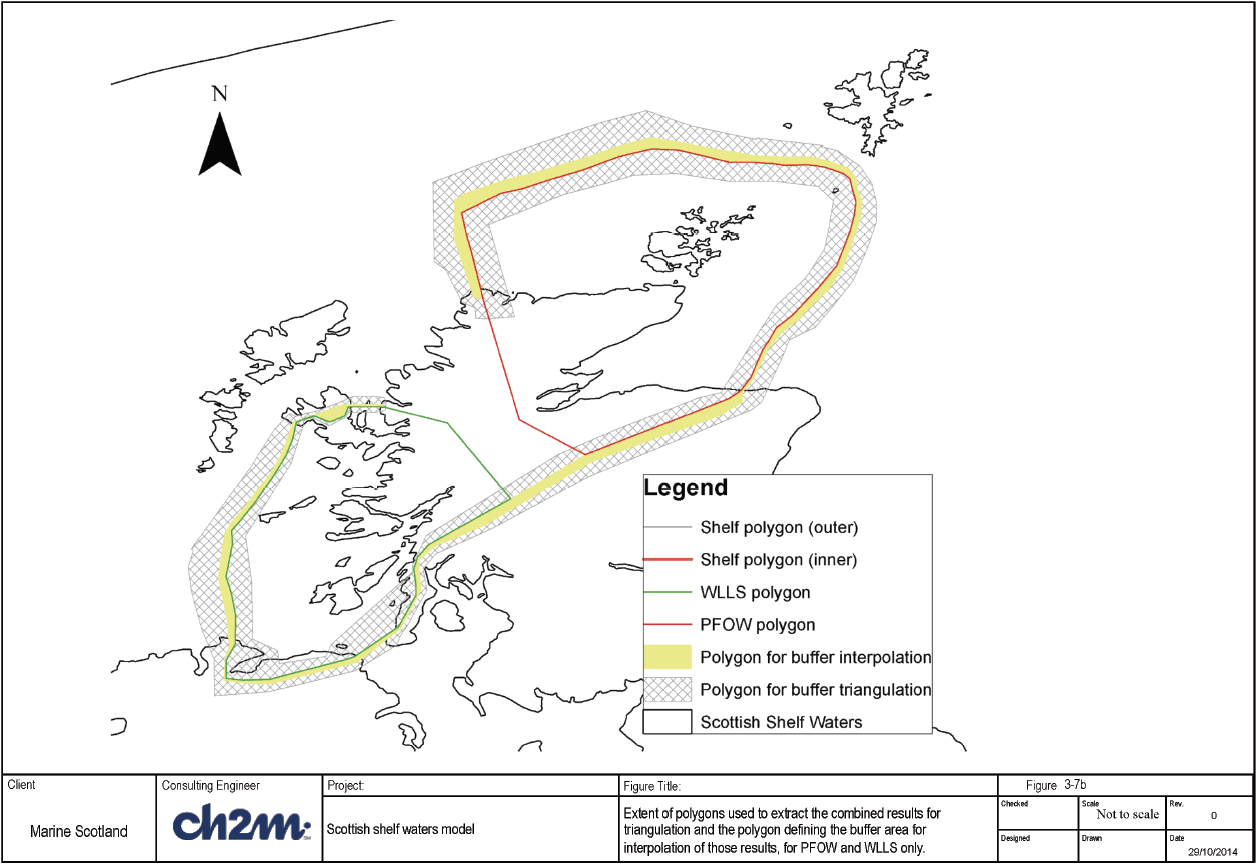
3) Interpolation weightings are also calculated for an interpolation buffer used later to smooth the transition between the various model results as shown in Figure 3-7a and b. The triangulation is carried out on the points within the inner and outer buffer polygons and the point location is carried out on the buffer polygon. Again, the nearest neighbour is also calculated in case any of the nodes or element centres fall outside the valid triangulation zone ( Figure 3-6a and b).

4) The header information and static variables are written to the NetCDF file.

5) For each time step the time dependent variables were interpolated from the shelf and local models into the new integrated mesh one model at a time, using the inpolygon function in Matlab to determine which nodes/elements to interpolate onto. The polygons are defined as shown in Figure 3-8. Note that the polygons for interpolation of the local model results follow the same line as the inside line of the buffer polygon and lie within the local model domain boundary. This is to avoid any issues at the boundaries being transferred to the particle tracking model and to ensure the buffering from the local models to the shelf model is successful.

6) In areas close to land where the "integrated" model mesh had a higher resolution than the local ("results") model mesh, the element centres of the "integrated" mesh will fall outside the valid triangulation of the local model element centres ( Figure 3-6a). In these areas the nearest neighbour function was used to avoid unrealistic results being passed into the particle tracking model. The areas where this was necessary were defined as a polygon and shown in Figure 3-9.

7) When all the model results have been combined the boundary between the different models is smoothed using the method described below:

a. Results either side of the interpolation buffer are extracted from the combined mesh ( Figure 3-7a and b).

b. The results on the nodes and element centres within the buffer are interpolated from the integrated results either side of the buffer and slotted back into the integrated mesh. Close to land where necessary the nearest neighbour value was used.

8) The interpolated results on the integrated model mesh are written to the NetCDF file at each time step. Daily input files are required for the particle tracking model, therefor the process was repeated for each day of the year.

3.4 Issues and solution

An initial attempt to develop the Matlab script for combining the results presented issues with unrealistic computational times and insufficient memory. The interpolation weightings calculations were performed as matrix calculations, meaning the interpolation weights for all nodes or elements could be calculated in one step, instead of looping through the nodes/elements one at a time, thus increasing the computational speed. Since the interpolation weights are calculated based on the geometry of the mesh, which is static, the interpolation weights were calculated prior to the interpolation of the results. This means the interpolation weightings for the nodes and elements only had to be calculated once and could then be used for all time steps and relevant parameters. Using the inpolygon function allowed the interpolation to be carried out only in the relevant areas of the mesh.

The polygon for the shelf model has an inner and outer boundary. This prevents results from the shelf model being interpolated to the S3 mesh in the areas covered by the local models only to be over written (when the results of each local model is interpolated to the S3 mesh), thus improving efficiency. The polygon for the PFOW model does not include the area of the SMB model, again preventing data being written to the same area twice.

The shelf model has 20 layers while the local models have 10 layers. To reduce computational times and memory requirements it was decided to reduce the number of layers in the shelf model to 10 instead of increasing the number of layers in the local models, due to the higher horizontal resolution in the local models. For parameters calculated on the layers the results were averaged using Equation 3-1 and for parameter calculated on the levels every second value was used.

(3-1)

The WLLS model has 10 variable thickness layers and 11 variable thickness levels, therefore to incorporate these results into the combined mesh it was necessary to interpolate the results on to 10 equally spaced layer and 11 equally spaced levels. This was carried out prior to running the script to save time. Since it is necessary to loop through all the nodes with the selected interpolation method it was quicker to do this for all time steps within a results file at once instead of looping through all the nodes and elements one time step at a time in the main script.

The issue of insufficient memory was tackled by reading in the model results, performing the interpolation and writing out the results to the NetCDF file one time step at a time.

Another issue was the realisation that around land the triangulation may not be valid and would produce unrealistic results. This would only be an issue when the results from a local model were being interpolated onto a higher resolution mesh. The issue was solved by defining polygons in which the results of the nearest neighbour is used ( Figure 3-9).