Priority marine feature surveys within the Small Isles MPA and surrounding waters
Marine Scotland collected and analysed abundance information for species with conservation importance relevant to priority marine features in the Small Isles MPA and the surrounding region (2012 – 2017). Abundance changes for key species and the relationship with fishing activity was assessed.
2. Methods Summary
This section provides an overall summary of the methods used to generate the Marine Scotland Small Isles MPA dataset (2012 – 2017) and to create this report. A comprehensive description of the methods is available in the full methods version provided in Annex C of the Annex Materials document (Greathead at al. 2023).
2.1 Baseline benthic monitoring
Imagery data in the form of DSI and HDV were recorded from 1) inside the areas covered by the proposed fisheries management measures; 2) inside the wider SMI MPA but outside proposed fisheries management measures; and 3) in areas outside the MPA boundary.
Imagery surveys used lander frames, which were set down on the substrate to collect DSI, and more traditional drop camera frames that drifted over the substrate at a fixed height. Lander frames had the advantage of offering a fixed focal length, producing stable images of a known area, but were not suitable for very rough ground. Time, depth and vessel position were recorded for both types of deployment, lander and drop frame. Annex B, Table B.1 (Greathead at al. 2023) summarises the year and month of each cruise and information on the equipment used. DSI and HDV footage were collected from both the lander and drop frame configurations. Due to differences in the survey design, only HDV were analysed in the drop frame configuration and only DSI were analysed in the lander configuration. The HDV collected by lander and DSI collected by drop frame were stored as back-up imagery data for habitat or species identification, if needed.
Depths surveyed ranged from 50 to 250 m (see Annex A, Tables A.1 and A.2 in Greathead at al. (2023)). Transects for HDV lasted a minimum of 10 minutes at a target speed of less than 1 knot, with mean tow speeds in the different survey boxes ranging from 0.32 to 0.96 knots (see Annex A, Table A.2). A minimum of three DSI stations were recorded in each transect (start, middle and end), with five DSI captured at each station.
There was limited prior information on the distribution of species and habitats over the entirety of the SMI MPA, thus surveys conducted during 2012 and 2013 served as scoping surveys that informed later refinements to the size and location of survey boxes. The 2012 and 2013 surveys used information provided by NatureScot and seabed morphological data from the ship's sounders to help draw the boundaries of potential survey boxes. Species distribution models (SDMs) produced by Marine Scotland for several PMF species or habitat components enabled the identification of viable survey areas not yet known to contain such records (e.g., Greathead et al., 2015; Stirling et al., 2016), further widening the area of survey. Over time, this process allowed the delineation of survey boxes that targeted the full range of PMF species or PMF habitat components thought to be present in the area.
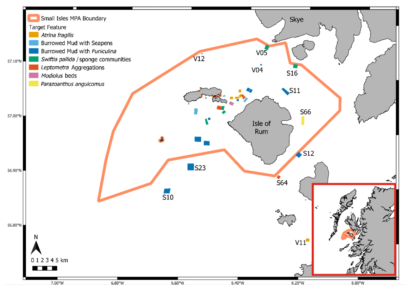
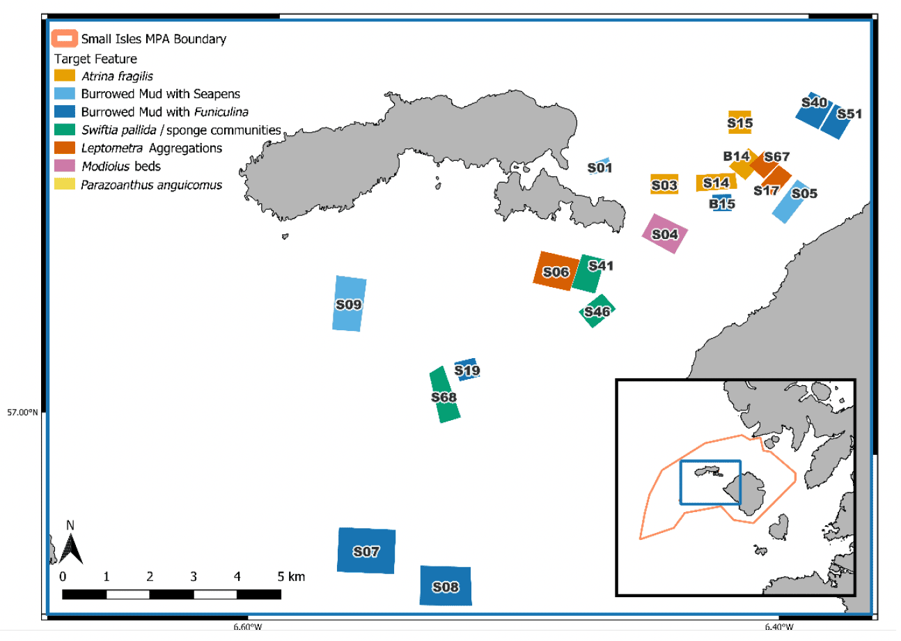
During the study period, some survey boxes were rejected if they did not contain target species or habitat or if they were too difficult or dangerous to survey. This approach resulted in the selection of 25 survey boxes from the original 31 for further survey (Fig. 3a, 3b). These 25 boxes were designed to survey ten features relevant to PMFs and were grouped according to different levels of future protection (inside/outside proposed measures and outside the SMI MPA) (Table 3; Annex A, Tables A.1 and A.2). More detailed notes on each research survey are contained in Annex B, Table B.2 (Greathead et al., 2023).
Survey boxes were subdivided by seven primary target features (BS: seapens, including Virgularia mirabilis and Pennatula phosphorea; BF: burrowed mud with Funiculina quadrangularis; MM: Modiolus modiolus beds; SC: Swiftia pallida communities; LC: Leptometra celtica; PA: Parazoanthus anguicomus; and AF: Atrina fragilis) and three secondary target features (BM: burrowed mud; BP: burrowed mud with Pachycerianthus multiplicatus; and AS: Arachnanthus sarsi) (Table 3). In addition to division by target features, survey boxes were also assigned to one of five major habitat types adopted for the purposes of survey design (soft sediment; mixed sediment; mixed sediment with cobbles; mixed sediments with cobbles and boulders; and cobbles, boulders and bedrock) and one of three site categories (inside/outside measures within the MPA and outside the MPA: see Table 3). Although it was not possible to find suitable survey boxes for each category, the survey design allows comparison between several possible categories inside/outside proposed measures or the SMI MPA for each target feature.
Table 3
Small Isles MPA survey boxes for ten target feature groupings, including: three priority marine feature (PMF) habitats, three biotopes of the burrowed mud PMF habitat, and four shellfish and other invertebrate PMF species (NatureScot, 2020b). Target features were distributed amongst five broad substrate types adopted for the purposes of survey design: soft sediment (SS), mixed sediment (MS), mixed sediment with cobbles (MSC), mixed sediment with cobbles and boulders (MSCB), and bedrock with mixed cobbles and boulders (CBR). Three site categories are identified for the target features: inside/outside management measures within the MPA and outside the MPA.
| Feature code | Target feature | Feature type | Substrate type | Survey boxes | ||
|---|---|---|---|---|---|---|
| Inside measures | Outside measures | Outside MPA | ||||
| BM | Burrowed mud | PMF habitat | SS | S06, S40 | S09, S17 | S10 |
| BS | Seapens and burrowing megafauna in circalittoral fine mud | PMF biotope of BM habitat | SS | S06, S40 | S05, S07, S08, S09, S11, S51 | S10, S64, S23, V11 |
| BF | Burrowed mud with Tall seapen (Funiculina quadrangularis) | PMF biotope of BM habitat | SS | S19, S40 | S05, S07, S08, S11, S51 | S10, S12, S23 |
| BP | Burrowed mud with Fireworks anemone (Pachycerianthus multiplicatus) | PMF biotope of BM habitat | SS/MS | S06, S15, S40, S67 | S05, S17 | S10, S12, S64 |
| MM | Horse mussel (Modiolus modiolus) beds | PMF habitat | MSC | S03, S04 | ||
| SC | Northern seafan (Swiftia pallida) and sponge communities, (occasionally with Caryophyllia smithii) | PMF habitat | MSCB/ CBR | S16, S41, S46, S68 V05 | S17, S66 | V11 |
| AS | Arachnanthus sarsi | PMF species | MS | S03, S15, S67 | S17 | S12, S64, V11 |
| PA | Parazoanthus anguicomus | PMF species | MSCB/ CBR | S06, S41, S46, S68 | S17, S66 | |
| LC | Leptometra celtica aggregations (on mixed sediment or Rock) | PMF species | MS/ MSC or MSCB/ CBR | S06, S40, S46, S67 | S17, S66 | S64 |
| AF | Atrina fragilis | PMF species | MSC | S03, S04, S15 | V11 | |
2.1.1 Species identification
Species identification was standardised using identification keys based on existing taxonomic works (Hayward and Ryland, 1990; Manuel, 1988) and modified to emphasise identification features that could be distinguished from digital formats. Electronic annotation (within Photoshop Elements 12) was used to ensure that each DSI could be re-analysed to confirm identification. All target species identified in the video transects were assigned a time code so that they could be easily found again for identification verification. Only features identifiable at a size of 10 mm or more were included in the analysis. Where smaller species were identifiable to genus level (e.g., Caryophyllia sp.), such species were classified if there was a high confidence in being able to consistently identify the feature.
The details of how taxa were identified and quantified from DSI and HDV imagery are available in the full methods, provided in Annex C.
2.1.2 Estimating species density
Species density estimates were derived from the two different survey methods employed over the course of the study; lander and drop frame. DSI quadrats were only used from the lander deployments. Due to its fixed focal length and angle, DSI quadrats from the lander frame produced a known "area under view" and were used preferentially in the survey of soft sediment habitats. The drop frame, which drifted approximately 80 cm over the seabed instead of "landing" on it, was used from 2015 onwards to record HD video across harder substrates where high levels of ruggedness precluded landing a frame. Obtaining HDV and DSI using the towed drop frame, although not as stable as the lander, also increased the area under survey over hard substrates.
The DSI area-under-view from the drop frame was not quantifiable and, therefore, these images were not used for analysis, but were used to verify species identification from the drop frame video transects. It should be noted that lander surveys in 2012, 2014 and 2015 also included areas of harder substrate, which from 2015 onwards were surveyed using HD video obtained from the drop frame. More information on the equipment used to collect imagery data across years is provided in Annex B, Table B.1; details on the imagery data types used to determine survey box-level density values for the different target species are provided in Annex A, Tables A.3 – A.10 of the Annex Materials document (Greathead et al., 2023).
The density of the eight target species was calculated at the survey box-level using a custom R-script (version 4.1.3; R Development Core Team, 2022), based on abundance within individual DSI quadrats or HDV tows and the total viewed area of seabed within each survey box for any given year and survey box combination. For seven species where detailed box level results are provided, density is reported as individuals or colonies within a metre squared (n.m-2); for P. anguicomus, density was reported as the number of occurrences (spatially distinct groupings) within a metre squared (o.m-2). More comprehensive details of how species density was determined from DSI and HDV imagery are available in the full methods, provided in Annex C.
To investigate whether survey box-level changes in density over time were statistically significant, a case study was produced using F. quadrangularis and S. pallida abundance data from a subset of survey boxes and years. The main results of this case study are presented under '3.1 Baseline Benthic Monitoring'; the full case study, including methods, is available in Annex D of the Annex Materials document (Greathead et al., 2023).
2.2 Assessing the impact of fishing activity on Funiculina quadrangularis abundance
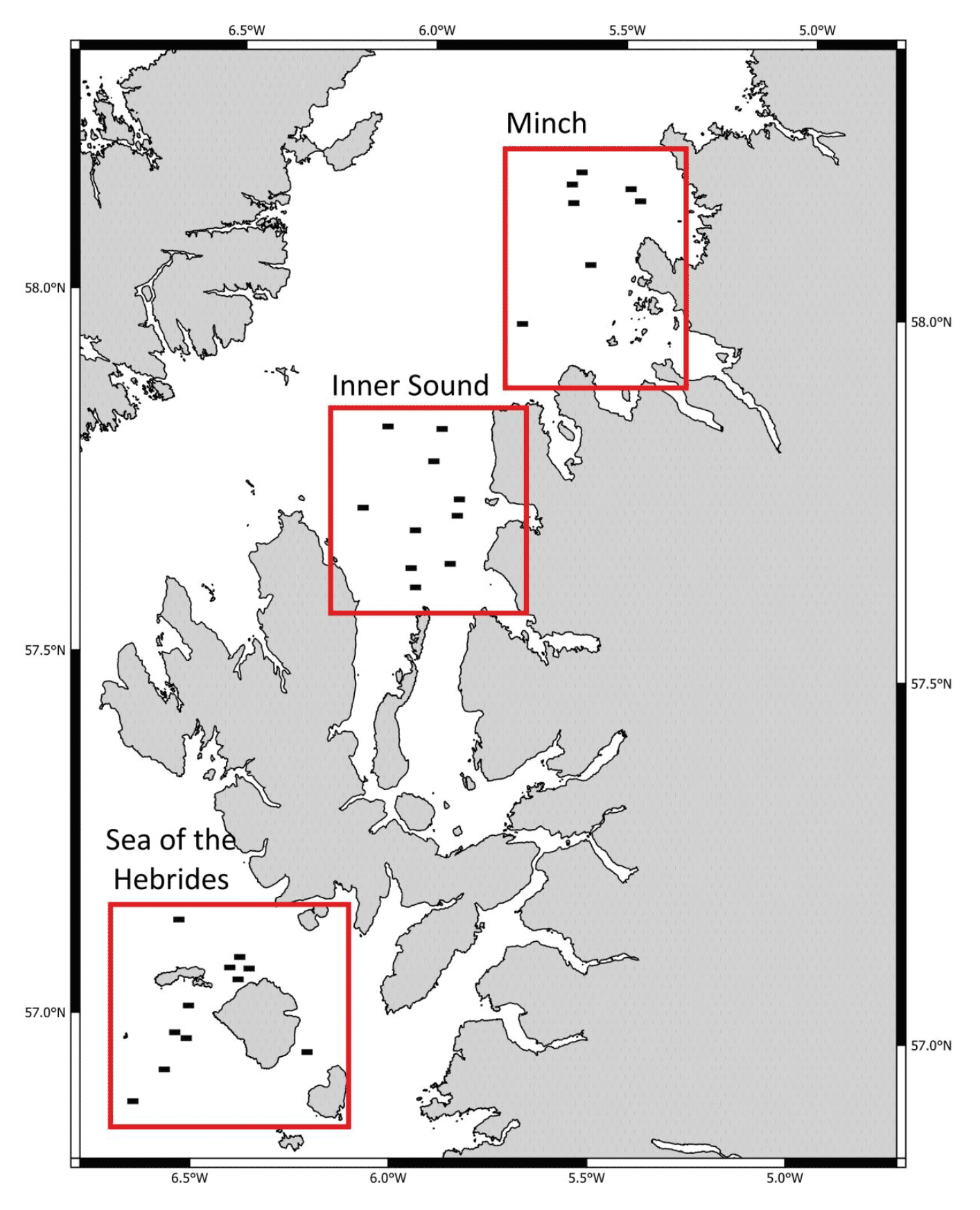
To assess the possible impact of fishing on the distribution of F. quadrangularis, a wider survey across three adjoining areas, the Sea of the Hebrides, the Inner Sound and the Minch was conducted in 2017. The survey areas were known to contain suitable substrates for F. quadrangularis, as indicated by species distribution models (Greathead et al., 2015) and confirmed during a subsequent Marine Scotland survey conducted in 2014. The survey areas were also known to vary in the intensity to which they were exposed to bottom-contacting towed gear.
To assess the effect of fishing intensity on the abundance of F. quadrangularis, study boxes across the wider West coast of Scotland were surveyed during September 2017 on the MRV Alba na Mara (Fig. 4). The 29 survey boxes with available vessel monitoring system (VMS) data were used for further analysis, with each study box being approximately 1.5 x 1 km in size. The survey adopted the lander methodology described earlier, using DSI quadrats to determine counts of F. quadrangularis. Within each survey box, a minimum of four transect tows of the lander were made. Conditions permitting, each tow would comprise of eight to ten stations of five DSI quadrat images. Quadrats within each station were placed according to the prevailing drift of the vessel and were all within 15 m of each other. This protocol aimed to collect a total of 30 – 50 stations (150 – 250 DSI quadrats) of known area in each box.
2.2.1 Deriving fishing intensity from Vessel Monitoring System data
A spatially resolved index of fishing intensity for bottom-contacting towed gear was derived from VMS data. Although VMS data presented the best available fishing data for the study period, it should be noted that there is no data requirement to collect VMS data for vessels shorter than 12 m in length and it is therefore an incomplete record. Fishing data for the years 2014 – 2016, the three years preceding the F. quadrangularis seafloor survey, were downloaded from the International Council for the Exploration of the Sea (ICES) website (ICES, 2018) on 9 March 2020. Swept-area ratios (SARs) were provided for both the seabed surface and subsurface; surface abrasion is defined as disturbance of surface features only (top 2 cm of sediment), and subsurface abrasion is penetration and/or disturbance of the sediment deeper than the surface of the seabed (≥ 2 cm). Due to F. quadrangularis being situated with three quarters of its body protruding above the sediment surface (Ager, 2003), and the nature of its interaction with towed fishing gear, only surface abrasion was included in subsequent analyses.
Further details on how fishing intensity was derived from VMS data are available in the full methods, provided in Annex C.
2.2.2 Environmental data
Environmental variables known to affect the distribution and extent of F. quadrangularis (Greathead et al., 2015) were included in subsequent analyses: bathymetry, percentage mud, sand and gravel, and salinity (Table 4). The bathymetry layer was then used to produce two additional environmental layers relating to the seabed - slope and curvature - using the spatial analyst and the benthic terrain model tools in ArcGIS.
Further details on how environmental data were derived are available in the full methods, provided in Annex C.
Table 4
Environmental variables considered in the Funiculina quadrangularis analysis
Variable: Depth
Description: High resolution (25 m2) digital terrain model of the subsea surface iteratively synthesized using high resolution multibeam bathymetry surveys.
Source / Derivation: SeaZone, 2013. Bathymetric Data historically supplied under licence 122006.004; data management tools in ArcMap 10.0.
Variable: Slope and curvature
Description: Derived from depth at the final resolution.
Source / Derivation: Depth and spatial analyst tools in ArcMap 10.0.
Variable: Sediment: mud (%), sand (%), and gravel (%)
Description: Sediment layers obtained after interpolation with inverse distance weighting, using the coastline as a barrier, grabs data from Marine Scotland and BGS.
Source / Derivation: Marine Scotland and BGS grabs; spatial analyst tools in ArcMap 10.0.
Variable: Salinity near bottom
Description: Minimum values calculated for the period 1988–2004 using R and resampled to the final resolution using the bilinear resampling algorithm tool.
Source / Derivation: POLCOMS model (Holt et al., 2005); R package "ncdf" (Pierce, 2011); and data management tools in ArcMap 10.0.
2.2.3 Statistical analyses
The effects of fishing intensity, depth, sediment, salinity, slope and curvature, and study area (Sea of the Hebrides, the Inner Sound and the Minch) on
F. quadrangularis counts (FQ count) within each station were examined within a Generalised linear mixed model (GLMM) framework within the R package, lme4 (Bates et al., 2015). The data were centred relative to the median before analysis. Preliminary modelling indicated that little between-quadrat heterogeneity existed in the covariates within stations, favouring the use of station level data due to the low number of counts per quadrat. The full fixed effect model structure was:
FQ count [Station] ~ area + depth + fishing intensity + % mud + % gravel + salinity + slope + curvature
Survey box and station were included as random effects (McCulloch et al., 2008). Random‐effects structures were compared with more parsimonious models within a GLMM framework that excluded the random effect component. Counts were modelled using a Poisson probability distribution with a log link function. Correlation between the explanatory variables was checked for collinearity using Spearman rank correlations and Variance Inflation Factors (Zuur et al., 2009). The full model was then simplified in a backwards stepwise procedure with model selection based on Akaike's Information Criteria (Akaike, 1974). The relative importance of each variable was assessed by a likelihood ratio test. Residual plots were examined for evidence of lack of fit or departures from the modelling assumptions. All statistical analyses were done in R (version 3.6.3; R Development Core Team, 2020).
Contact
Email: rachel.boschen-rose@gov.scot