Flood prevention schemes: guidance for local authorities

SECTION 3: MORE SPECIALISED TOOLS AND TECHNIQUES

Introduction

3.1 The risk register approach described in the previous section should be the first step in risk analysis. However, many areas of risk assessment are only partly covered by such an approach. Particular risks may require more specialised methods of analysis. A decision to use such methods will be influenced by a number of factors, including the following:-

• A meaningful investment appraisal will often require detailed, quantitative, analysis of risks and uncertainties. For example, assessment of breach probability by quantitative analysis of the loads, such as water levels, waves, and the strength of the structure.
• Systems may be complex with interactions that are not easily dealt with by the risk register.
• Some risks may have common causes of failure which can only be addressed by more sophisticated methods.
• The balance between different types of impact may need to be considered in more specialised ways.
• Uncertainty may need to be reduced by more detailed investigation and analysis.
• Appraisal needs to consider changes over time, many years into the future, and more complex approaches may be required to track the changes in time, and to analyse decisions required now and in the future.

3.2 The results of the more specialised methods may be fed back to the risk register - in terms of (i) more reliable and accurate estimates of likelihood and probabilities, (ii) design or justification of mitigation measures, or (iii) review of the risks identified and more complete descriptions of their occurrence and interactions.

Event and fault trees

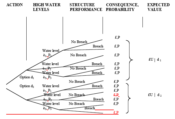
3.3 Event and fault trees are a primary tool for understanding the components of a problem, and combining probabilities in a logical manner. A diagrammatic example is shown in Figure 3.1. Here, a decision between options involves a range of possible consequences depending on (i) the maximum high water level encountered, and (ii) the performance of the structure during that high water event. In the example, the structure performance is represented by the probability of a breach developing. The expected value of each option can be calculated reflecting the probabilities and consequences of the outcomes.

Figure 3.1 Decision/event tree for comparing options with uncertainty

Multi-criteria approaches

3.4 It is often assumed that the consequences of adopting any option can be condensed to a single, usually monetary, value. This is the situation addressed in economic appraisal of projects, and will be the most usual context in which risk-based decision-making is adopted. For large-scale planning decisions, and during early stages of strategy development and project appraisal, it may not be possible or appropriate to express all of an option's attributes on a single, economic scale. Under these circumstances, so-called multi-criteria or multi-attribute methods can help in screening all the options. They can also help to build consensus between project participants who may have divergent objectives.

3.5 A multi-criteria matrix is illustrated in Table 3.1. The performance of each of the options d ₁, d _2,... d _l is scored against criteria A ₁, A ₂,... A _n. Thus the score of option d ₁ against criterion A ₁ is a ₁₁, and so on. If a weight is applied to each of the attributes, a unified score for each of the options can be computed. This forms a basis for selecting the preferred option or, perhaps more often, to screen out those options which are not worth pursuing further.

Table 3.1 Multiple criteria matrix

		Criteria	A 1	A 2		A n
	d 1		a 11	a 12	…	a 1n
	d 2		a 21	a 22	…	a 2n
			.	.	…	.
			.	.	…	.
Options
			.	.	…	.
	d l		a 11	a 12	…	a 1n

3.6 Since multi-criteria methods are most usually applied at the large-scale planning stage, or during pre-feasibility studies, information relating to the future performance of options is at its most scarce, and uncertainty at its most acute. Uncertainty may be accounted for by defining criteria against which an option can be judged. For example, environmental impacts might be simply scored: 1 (no impact), 2 (medium impact) or 3 (high or unknown impact). Another approach is to incorporate uncertainty as a criterion. For example, in relation to flooding, a simple scoring system might be: 1 (low uncertainty - over 30 years of records and validated modelling); 2 (some uncertainty - less than 30 years of records and limited modelling); or 3 (high uncertainty - very limited data available).

3.7 Where the uncertainty in the scores applied to each option is great, it may be appropriate to assess the options under a range of different possible future states of nature T ₁,T ₂, . . . T _m. This will extend the table into a third dimension, which can be readily achieved using spreadsheets.

Sensitivity testing

3.8 Sensitivity testing is most useful when used to demonstrate the robustness of a preferred option. It involves examining a number of scenarios without attaching probabilities. Nonetheless, it enables an initial study of the potential consequences of uncertainty in future performance. It will often be appropriate to conduct some sensitivity tests before embarking on more thorough probabilistic methods.

3.9 Sensitivity testing can be used to assess the extent to which key variables can change before a different preferred option is identified. The likelihood of that change actually occurring will then require some judgment. Sensitivity testing usually involves varying each parameter in turn, with other parameters set at their 'best estimate' values.

3.10 The findings of sensitivity tests will therefore give a rather uncertain indication of the robustness of a preferred option. Further probabilistic analysis will often be justified for those aspects shown to be critical to decision-making.

Assessing probabilities

Introduction

3.11 Probability can be defined in many ways. The probability of an outcome is the relative proportion or frequency of events leading to that outcome, out of all possible events. For some systems, such as a lottery draw, or the throwing of dice, probability can be calculated directly and precisely from the properties of the system. For other systems, such as the weather, it is not possible to define all discrete conditions or states. The probability of rain cannot be calculated directly, but must be estimated in some way, from data, or modelling, or both. The probability will be approximate, not exact.

3.12 Probabilities may change with time; for example, due to climate change. It is worth noting that probabilities themselves may be uncertain, and that a range of probability values may need to be examined for sensitivity purposes.

3.13 The 'encounter' probability is useful for communicating risk levels. It is less likely to be misunderstood than return period. It can be calculated from the equation,

P = 1 - (1 - 1/T) ^N

where P is the probability, T is the return period of the design flood in number of years, and N is the particular time period of interest, also in number of years. For example, for schemes designed to withstand a flood with a return period of 100 years, there is a 0.63 probability (or 63% chance) that the design flood, or a more severe event, will be encountered within a period of 100 years.

3.14 Risk based decision-making requires a set of probabilities describing the relative likelihood of a range of future scenarios. This may entail:

• a model of the system of interest (paragraphs 3.15-3.18);
• some input probability distributions (paragraphs 3.19-3.21); and
• a method of integrating such distributions into the model (paragraphs 3.22-3.2.25).

Modelling the system

3.15 Understanding the system under appraisal, particularly its possible modes of failure, is an essential aspect of any risk assessment. Analysis by experts will be the starting point, often resulting in sketches of potential failure mechanisms. Although it may not prove necessary or possible to analyse them all, it is important to state the mechanism explicitly before excluding it from further analysis. This process is in many ways analogous to the generation of a risk register (section 2).

3.16 Having described the behaviour of the system in qualitative terms, it is necessary to develop a model suitable for quantitative analysis of probabilities. Fault tree analysis has proved its effectiveness in many disciplines. It involves identifying a specific state of a system (usually a failure state), and analysing all ways in which it can be reached. This type of analysis is particularly useful for mechanical and electrical systems such as floodgates, where components are fitted together in a clearly identifiable way, and where statistical failure rates are generally well documented. It enables critical elements to be identified and, if necessary, reinforced or duplicated, to improve the reliability of the whole system. Fault trees are therefore suitable for analysis of some aspects of flood defence systems. They are less applicable where failure mechanisms interact and are characterised by progressive cycles of decay rather than by discrete failure events.

3.17 Rather than working back from a defined failure mechanism (as in fault tree analysis), the overall behaviour of a system can be analysed by working through the events which may occur due to the loads on the system. This approach is particularly useful where there are only one or 2 key loads. In flood engineering, a statistical distribution of the key hydraulic loads will usually be available. This can be used as a direct input for a quantitative event tree analysis.

3.18 Event tree and fault tree analyses address failure at a particular point in time. However, the system will also be subject to long-term changes due to materials decay, embankment settlement, and the variation of the loads themselves. It is important to address such changes in an appraisal. This can be achieved by (i) analysing system failure at several discrete moments during the life of the scheme and interpolating; and (ii) simulating the behaviour of the whole system over the life of the scheme and directly obtaining whole-life predictions.

Obtaining input probability distributions

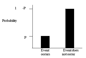
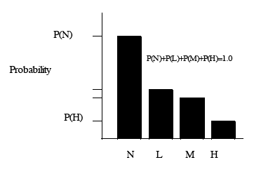
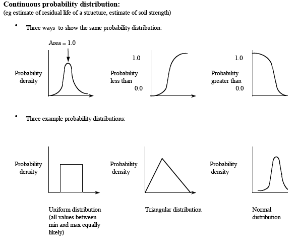
3.19 A quantitative risk analysis requires input probability distributions for the model. For example, for flood prevention schemes in tidal areas, this may require probability distributions for wave heights and tide levels. Distributions can be discrete (Figure 3.2), or continuous (Figure 3.3).

Figure 3.2 Examples of discrete probability distributions

Event probability: eg likelihood of unforeseen ground conditions during construction is low, or 5%.

Discrete probability distribution: eg probabilities of None, Low, Moderate and High flood severity at a site within the next year.

Figure 3.3 Examples of continuous probability distributions

3.20 Most analyses will have more than one input distribution. The correlation between the input variables should always be explicitly considered, even if only in a summary statement that they are independent. In some circumstances, such as waves/tide levels at the coast, and waves/tide levels/fluvial flows in estuaries, the input distributions will not be independent. Estimation of joint distributions may be required (reference 22).

3.21 In the development of probabilities it is important to (i) include all possible events and always confirm that the total probability equals one; (ii) be clear whether probabilities are conditional on other events (eg probability of breaching may be conditional on a given high water level); and (iii) always consider whether probabilistic variables are dependent and use the correlation where appropriate.

Integrating probability distributions

3.22 In a deterministic analysis of a system, a unique set of input parameters is used in the model to obtain a unique value for the system response. In a probabilistic analysis, a full range of input values is tested, each one weighted by the probability of it being encountered. The analysis should consider every possible input condition likely to make a significant contribution to the response. This requires a method for integrating the contributions.

3.23 In some cases, it is possible to use analytical methods of integration. The scope for such methods can be extended by making assumptions about the form of the relevant distributions at the point where the system will fail (reference 23). However, numerical methods are of more general applicability. There are 2 categories: (i) methods based on approximating the continuous input distribution as a discrete distribution, and systematically working through every discrete input condition; and (ii) methods based on random sampling from the input distribution ('Monte Carlo integration').

3.24 Monte Carlo integration proceeds by conducting a large number of realisations of the model, each one with randomly sampled input parameters. In each realisation, a single point is selected at random from the input distribution. The system response to these input conditions is then calculated. Thus, each realisation is a conventional deterministic analysis. By repeating the process many times, taking values from the whole range of inputs, the output distribution is built up. The accuracy of the method depends on the number of simulations performed. As the number increases, the output distribution converges towards that which would be obtained with an analytical integration, if such an integration were possible.

3.25 It is important to state explicitly the assumed correlation between input variables. The supporting evidence for the assumptions should also be stated.

Use of probabilities from expert judgment

3.26 While it is preferable to use probabilities derived from quantitative or statistical analysis, there may be situations where this is not possible and an element of expert judgment is inevitable. Even a seemingly quantitative statistical analysis is based on judgments, in respect of the data to be admitted and its applicability to the particular problem.

3.27 There is an ample literature to show that expert judgments, and specifically subjective judgments of probabilities, can be prone to bias. In project appraisal, it is important to avoid such bias as far as possible. Good practice guidelines are:

(i) Precisely define the events to which the expert is being asked to attach probabilities. The analyst should ensure the expert is attaching an accurate meaning to the event for which a probability is being elicited. It should be made clear whether exceedance or encounter probabilities are being sought. The distinction between cumulative probabilities over a number of years and annual probabilities should also be made clear. Similarly, if the probability of failure is being considered, the circumstances that constitute such failure should be carefully defined. For example, depending on the circumstances, this could be the first crack in a flood wall, the onset of wave overtopping, or the initiation of flood damage to property.

(ii) Structure the problem logically with the help of event trees. In complex situations, it will be very difficult for experts to handle the multiplicity of factors which determine the probability of system failure. It is often preferable, therefore, to decompose the problem using event trees, and to seek expert judgment on the constituent scenarios.

(iii) Use any available quantitative data to inform the expert judgment. In many studies, even if a full probabilistic analysis is constrained, there is often some statistical data which should be incorporated in the analysis. For example, it is usually possible to obtain statistics for the occurrence of extreme storms which initiate defence failure. This information can be used at one node in an event tree, and the expert can then be asked for the conditional probability of failure given that a specified storm or number of storms has occurred.

(iv) Check the expert testimony for inconsistencies. By logically structuring the probability information being requested, and obtaining several judgments on different aspects of a problem, it is possible to check for inconsistencies in the expert testimony. Where discrepancies are found to exist, work with the expert to develop a more coherent set of probabilities.

(v) Make use of peer review. Judgments should be subjected to critical review by the expert's peer group. The effort and cost of these reviews increases with the rigour of the method and the number of experts involved.

(vi) Document all the evidence upon which the expert judgment was based. Expert judgments of probabilities are based on evidence, which will range from specific analysis, data and historic evidence for the particular site, to the tacit knowledge of the expert. The expert judgment should, as far as possible, be made transparent by documenting the sources of evidence, and the associated processes.

(vii) Use expert judgments of bounds on probabilities or 'most likely', 'best' and 'worst' estimates rather than point estimates. Experts in flood engineering will themselves willingly acknowledge the uncertainty inherent in probabilistic predictions. This should be expressed in terms of a probability distribution (often based on 3 estimates: 'most likely', 'best', and 'worst'. Alternatively, the bounds on the estimate may be treated separately in the analysis, to indicate the sensitivity of the final decision to the expert's uncertainty.

Probabilistic discounting

Introduction

3.28 Much of the uncertainty in flood engineering relates to events which are likely to occur in the future, but the exact time is far from certain. Situations of this type are well suited to probabilistic treatment.

3.29 Uncertainty in the timing of a future event, can be a significant issue in economic terms. A good example is the impact which the residual life of a flood defence can have on the economic appraisal of the 'do nothing' option. If the residual life is short, a variation of only a few years can radically change the economic case for replacement. Yet experienced engineers will readily admit potential variability in residual life estimates. Under these circumstances, it is advisable to treat predictions in probabilistic terms. This involves establishing a probability distribution of the year in which a critical event will take place, and using this in a discount table. The approach is therefore known as probabilistic discounting.

3.30 The following caveats should be borne in mind:

• Probabilistic methods may give similar results to a deterministic approach, depending on the degree of variability; the skewness of the response and the spatial distribution of consequences (benefits); and the relationship between damage cost and flood severity. Such methods may be significantly more realistic if the benefits are dominated by a small number of high value assets.
• Probabilistic methods as outlined here produce expected values. These may be weighted to reproduce aversion to high consequence events. But in the final analysis, the decision criteria are generally based on single values of (expected) costs and benefits. In some cases, it may be more appropriate to examine alternatives to expected value criteria, such as multi-criteria methods, or to make several assumptions and discount each one separately.
• Probabilistic methods are best suited to processes that conform to random behaviour. The analysis is also used for other types of uncertainty, such as physical parameter and model uncertainty, but is not well suited to types such as 'incompleteness'. While experts are often employed to estimate probabilities, it should always be borne in mind that the results are to a degree artificial, reflecting strength of belief rather than a 'real world' probability.

Recurrent flooding events

3.31 Flooding is the most familiar type of event whose timing cannot be predicted precisely. The well-established approach of using a loss-probability curve (Chapter 5) is essentially a risk-based technique. This provides an estimate of the expected damage for the year in which the evaluation took place.

3.32 There may be a long-term change in the expected damage. For example, where a flood prevention scheme is being designed to alleviate fluvial/tidal flooding, the probability of damage behind the defences, due to overtopping, may increase due to expected sea level rises. In that situation, damages should be evaluated at several different points in the future, and these should be input into a discount table.

3.33 Under some circumstances, there will be a high degree of uncertainty associated with the predictions of expected damage. It will, therefore, be advisable to use a range of different estimates and discount each one separately. Probabilistic treatment of this uncertainty will seldom be justified.