Seabird flight height data collection at an offshore wind farm: final report

2. Methodology

2.1 Survey Planning

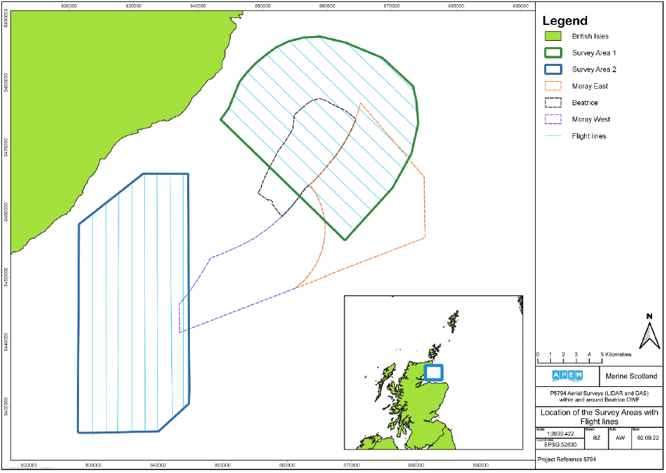
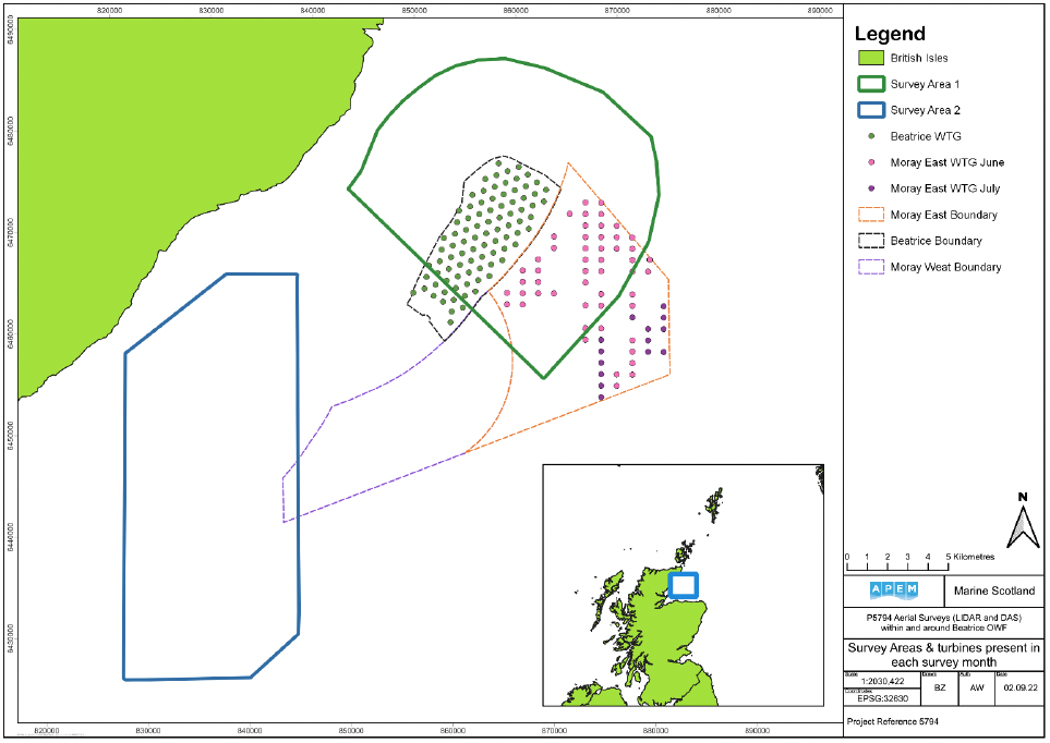
Data were collected within and around three OWFs within the Moray Firth, off the northeast coast of Scotland; Beatrice, Moray East and Moray West (Figure 1). At the time of the survey Beatrice had been operational for two years, Moray East was under construction and partially commissioned with 52 turbines present during survey 1 (June 2021) and 66 during survey 2 (July 2021). Moray West was consented, but no construction was underway at the time of the surveys.

APEM's bespoke combined high-resolution aerial digital stills and LiDAR system (herein referred to as imagery-LiDAR system), was fitted into a twin-engine aircraft and operated alongside a high accuracy positioning Inertial Measurement unit (IMU).

The survey flight plan was designed in advance using specialist flight planning software and included 13 transects spaced two kilometres (km) apart across Survey Area 1 and 9 transects spaced two km apart across Survey Area 2. These lines were flown for each survey to deliver a minimum coverage of approximately 10% (Figure 1). The aircraft collected these data at an altitude of approximately 450 metres (m) whilst travelling at a speed of approximately 120 knots. Flying at this altitude allowed for aerial digital survey data to be collected at an average of two centimetres (cm) ground sampling distance (GSD) allowing a high level of identification of seabirds from the digital still images. A Global Positioning System (GPS)-linked bespoke flight management system was used to ensure the tracks were flown with a high degree of accuracy and image capture points were recorded to allow birds to be accurately located within images. Additional survey lines were captured onshore over Wick where measurements of ground elevations had previously been made. These ground measurements were used to ensure high accuracy LiDAR point clouds were produced across the survey zone.

The first aerial imagery-LiDAR survey took place across two days, on the 15^th and 16^th June 2021, whilst the second survey took place on 15^th July 2021. The surveys were completed by a single aircraft with approximately eight hours on-task for one survey.

No health and safety issues were reported during the surveys.

2.2 Survey Timings and Conditions

2.2.1 Survey 1

15/6/21

For the first survey 19 of the total 22 transects were completed during the first day of data collection. As unsuitable weather approached before the final three transects were flown, the remainder of the survey was postponed until the 16^th of June. The cloud cover during the survey was classed as overcast. Visibility started at 20 km, before reducing to three km at the end of the survey. Winds were recorded at between six–20 knots from a southerly direction, with a sea state of zero–two (calm [glass] – smooth). The outside air temperature was recorded as 10°C.

16/6/21

The remaining three transects of Survey 1 were completed on the 16^th June. The cloud cover was classed as overcast, with a visibility of three km. Winds were recorded at 20-23 knots from a southerly direction, with a sea state of two–three (smooth to slightly moderate). The outside air temperature was recorded as 16°C.

2.2.2 Survey 2

15/7/21

All 22 transects were completed. The cloud cover was classed as 20% (scattered), with visibility at >10 km for the duration of the survey. Winds were recorded at 9-20 knots from a westerly direction with a sea state of zero (calm [glass]). The air temperature outside was recorded as between 10-16°C.

2.3 LiDAR Calibration

Prior to each survey technical calibration reviews were carried out to ensure both the high-resolution aerial digital stills system and LiDAR were set up to collect optimal data. This allowed for the most accurate data to be collected, processed and verified. Two main quality control stages were utilised:

1. System calibration: this is carried out when the LiDAR system is installed in an aircraft and is valid for the duration of that installation. APEM use a calibration site in Stoke.

2. System verification: this is carried out during the survey itself, by collecting data over highly accurate, ground control points (GCP's), both on the way out to the survey area and again on the return. APEM used a grid of GCP's in Wick for this survey.

Details of each control measure are outlined below.

1. System Calibration

A system boresight calibration survey was carried out by APEM at a pre-existing site in Stoke-on-Trent, England once the LiDAR system was installed into the survey aircraft.

The pre-existing site consisted of a grid of measured XYZ coordinates of fixed features on the ground. During the calibration set-up, the XYZ coordinates were surveyed using a high-accuracy, real-time kinetic positioning global navigation satellite system (RTK GNSS) 'smart rover' with accuracies better than 2 cm. The onshore data were used to calibrate the system to ensure accurate outputs were produced.

The system calibration computes the final offsets and lever arms between all of the system components to allow for production of high accuracy datasets.

During the flight, the Inertial Measurement Unit (IMU) creates trajectory files which records the position of the aircraft / sensor throughout the duration of the survey. The raw trajectory data from the calibration flight were post-processed using the single base function within Applanix POSPac v8 software which resulted in the position of the sensor to be known to a high degree of accuracy throughout the flight.

2. System Verification

The system verification check uses ground measured elevation data to compare against LiDAR data captured over a pre-existing site. For this project, a Ground Control Area (GCA) was established on a flat area of hardstanding in Wick prior to aerial survey. The GCA involves measurement of the XYZ coordinates of a grid of points spaced 50 cm apart over an area of land 500 cm x 500 cm. The XYZ coordinates were measured using an independent RTK GNSS Smart Rover with accuracies of less than 2 cm. During the flights, survey lines were flown over the verification site at the start and end of the mission. Elevations from the processed LiDAR data from these lines were then compared against the GCAs to assess the accuracy of the LiDAR data. One survey line was flown during the June survey due to inclement weather and yielded an accuracy of 1.8 cm Root Mean Square Error (RMSE). Two lines were captured during the July survey and returned an accuracy of 7.6 cm and 9.3 cm.

2.4 Data Processing

All of the high-resolution aerial digital still images collected were georeferenced using the geographical data derived from the GPS-linked bespoke flight management system. A GPS log was recorded during the survey flights, with GPS positions recorded at the start and end of each line flown and for each image captured throughout the survey. These data were uploaded into GIS to generate flight log shapefiles to represent the flight lines flown and the image nodes captured.

2.5 Image Analysis

The high-resolution aerial digital still images were analysed by trained ornithologists to detect the presence of seabirds. Using APEM's bespoke image analysis software the images were georeferenced, and the spatial locations were accurately determined for any birds in-flight.

Birds detected in the high-resolution aerial digital still imagery were identified to species level, where possible, by experienced ornithologists. Every bird recorded on these surveys was viewed by at least two members of staff as part of our comprehensive quality assurance (QA) process. Blank image QA was performed on at least 10% of the imagery to ensure no birds were missed. Finally, all bird identifications were checked by an experienced QA manager at APEM.

Once the image analysis was complete, APEM's BIRD software automatically generated a tabulated database containing information corresponding to each individual sighting including group / species, geographical position of the individual, timing of the sighting and behaviour (flying, sitting, submerged etc.). The database was exported into Excel format to provide simple raw count-based data. Taking the positional information stamped to each sighting, the sightings were plotted directly into a GIS to create shapefiles, whereby each sighting is represented by a single point. The digital nature of both the outputs (tables and shapefiles) enabled both a statistical and spatial statistical analysis to be performed on these data.

2.6 LiDAR Analysis

The data collected from the LiDAR system was output as a database of the point cloud with each point having a XYZ coordinate. The processed LiDAR point clouds were then loaded into specialist LiDAR analytical GIS software, along with the shapefile of flying bird locations identified and tagged during image analysis.

Analyses were carried out to identify points in the point cloud above the sea surface that correspond to the approximate location of the same bird in flight within the high-resolution aerial digital still imagery. The size and behaviour of the bird (gliding / banking / diving [Appendix VI]) can impact how many hits or returns the LiDAR is receiving from a given individual.

Birds with two or more hits were assumed to be highly accurate. Birds with a single hit were assigned a confidence category of "high" or "low". This is because single hits could also be representative of noise in the point cloud. Noise is a common phenomenon in all aerial LiDAR datasets and is usually attributed to moisture or other significant particulates in the air and can be caused by rain, fog, low clouds, ocean spray, or even large insects. It manifests itself as apparent random points above the normal surface of a point cloud and can be over 100 m high.

2.6.1 Flight Height Less Than Two Metres

The matching process does not change for low flying birds (less than two metres above the water surface). The tagged bird locations are identified in the LiDAR data and all above surface "object" points extracted from the point cloud. The successful mapping of the sea surface means the number of potential false positives was reduced, even close to the surface. Under rougher sea conditions, the amount of noise around the surface is likely to increase. However, under APEM's methodology the imagery is used as the primary source of data for bird identification and the LiDAR matched to the data from the imagery. Therefore, noise from the sea surface was not expected to have a significant impact on the overall results.

When considering these data during the matching process, a single isolated LiDAR point above the surface in close proximity to the tagged bird location can be matched with high confidence.

A single hit close to a bird, but with other single hits (noise) in the vicinity, was assigned to a low confidence score. In general, there may be instances where no match can be made as there are too many noise points to match a bird even to a low degree of accuracy or there are no points in the cloud to match to. This may be caused by the movement of the bird reducing the surface area available for the LiDAR to bounce off or the bird flying too low to the surface to be distinguishable from waves / sea spray during certain conditions. Despite this, no lower cut-off value is enforced for flight heights when birds are close to the sea surface, as success with matching is still made possible by the supporting high-resolution aerial digital still imagery.

2.6.2 Data Set Matching

Once the LiDAR data were matched with birds from the high-resolution aerial digital still imagery, the average flight height for each individual was extracted from the corresponding LiDAR cluster and assigned to a master shapefile. This process then produced a record of each bird species, heading, age, size, geographic coordinates, flying height (metres) relative to base datum and flying height above the sea surface in metres. The number of hits per bird were also recorded in the master shapefile. All species groups with more than one count had a match rate of better than 81% (Appendix II).

2.7 Data Analysis

All data manipulations and analyses were carried out in R (R core team, 2022). GIS software (QGIS) was used to create maps and present spatial data.

The raw counts of birds found in each survey month (survey 1=June 2021, survey 2=July 2021) were collated in tables and distribution maps. The data for the current study was collected by APEM at two different study locations (Survey Area 1, and Survey Area 2, Figure 2). The locations were defined as follows:

Survey Area 1:

• Beatrice, covering birds recorded within the Beatrice OWF boundary.
• Moray East, covering birds recorded within the Moray East OWF boundary.
• Survey Area 1 without OWFs, which covered all areas of Survey 1 that did not overlap with the Moray East and Beatrice OWFs.

Survey Area 2:

• Survey Area 2, covering the control survey area without any WTGs.

2.7.1 Comparing flight height in the different study areas

The flight height of birds in areas with WTGs and without WTGs were compared. A visual comparison between Survey Area 1 with WTGs and Survey Area 2 without WTGs is shown in a violin plot for the following species which are of high risk of collision; fulmar (Fulmarus glacialis), gannet (Morus bassanus), large gulls (Larus argentatus and Larus marinus) and kittiwake (Rissa tridactyla) for each survey month. Additional statistical analysis was performed to compare the flight height in the different study areas for the species of interest. A non-parametric two-sample Mann Whitney U test or Wilcoxon rank sum test was performed for each species and for the species combined.

Histograms of distance to nearest turbine (m) were created for each species detected in survey 1 and survey 2 (Appendix V), using the ggplot2 package in R. The script used is available in Appendix IV.

2.7.2 Modelling fight height in relation to WTG distance

The flight heights of the birds were modelled in relation to the distance to the closet WTG in Survey Area 1 using linear and mixed models in R.

The distance for each recorded bird to the nearest WTG was calculated in QGIS. WTG data were altered to only include those that were in situ at the time of each survey in June and July 2021.

Histograms of the flight height relative to sea surface level showed that these data were not normally distributed. To account for these data distribution, we used Box-Cox transformation for the mixed models. The R script used is available in Appendix IV.

For the statistical modelling the lme4 package was used (Bates, et al. 2015). The height relative to sea level measured by the LiDAR system (BirdZ_SeaL) was analysed, using 'distance to the nearest WTG (m)' as a continuous variable with a fixed effect. The different survey months were included as a random effect. Additionally, the main species were analysed together, and common name included as a random effect.