Publication - Research and analysis

Seabird flight height data collection at an offshore wind farm: final report

Published: 30 September 2022
Directorate: Marine Directorate
Part of: Environment and climate change, Marine and fisheries
ISBN: 9781804358771

Understanding seabird flight heights and behaviour in and around operational offshore wind farms is a priority knowledge gap. Using aircraft mounted LiDAR technology, this study collected data on seabird flight height and shows the potential for using it in offshore windfarm impact assessments.

Supporting documents

Appendix IV. Model diagnostic plots and full model outputs

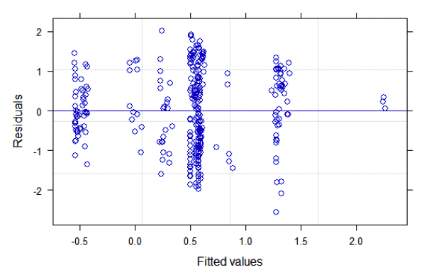
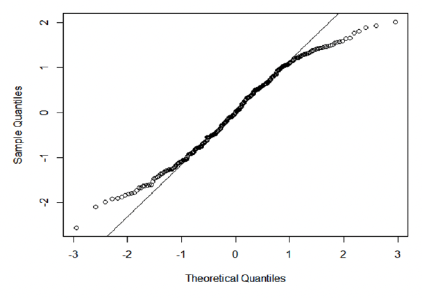
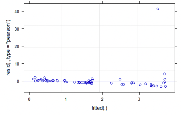
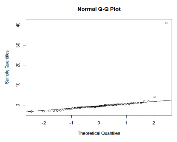
Modelling fight height in relation to WTG distance (all species combined)

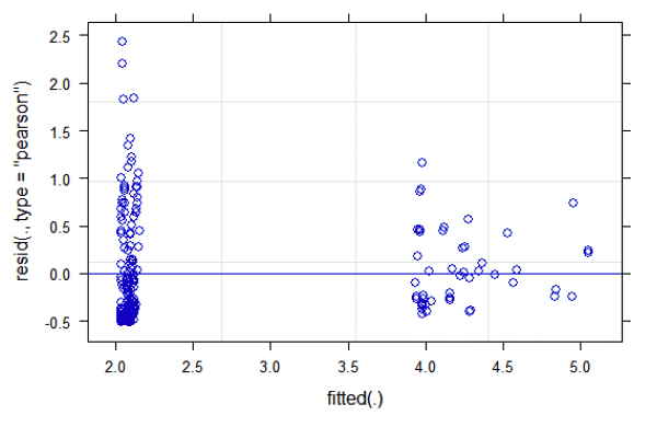
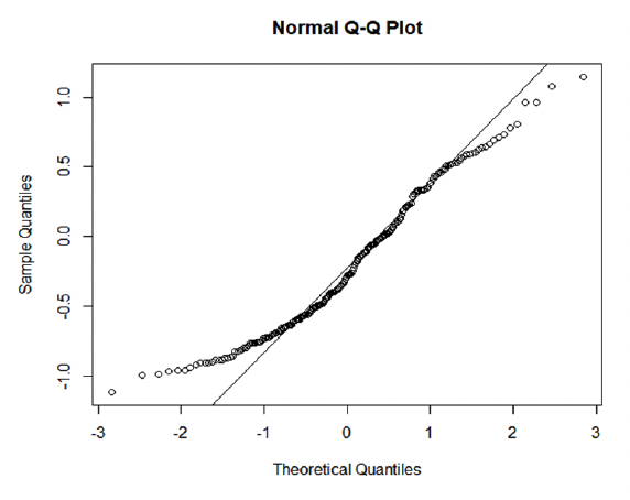
A scatter plot for all species combined with residuals on the y axis ranging from 2 to -3 and fitted values in the x axis ranging from -0.5 to 2.0. There are dense clusters around -0.5, 0.5 and 1.3 fitted values, with the residuals evenly distributed in a range from 1.5 to -1.3, 2 to -2, and 1.2 to -2.7 respectively — Figure IV.1 Plot of the LMM for both survey months in Survey Area 1.

A normal Q-Q plot with sample quantities on the y axis ranging from 2 to -2 and theoretical quantiles in the x axis ranging from -3 to 3. The line of best fit starts from -2.4 theoretical quantiles and extends up to 1.7 — Figure IV.2 Q-Q line plot of the LMM of flight height against distance to the nearest turbine.

Kittiwake

Fulmar

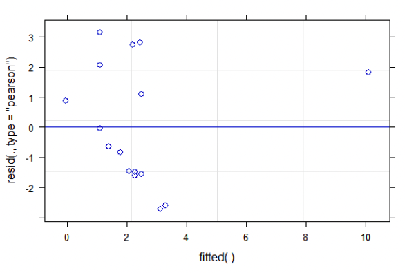
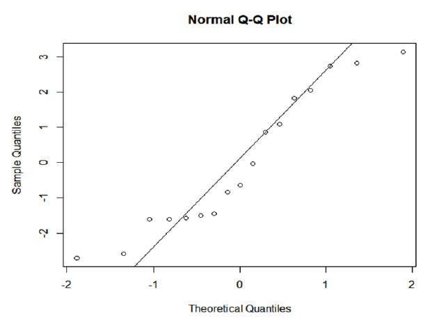
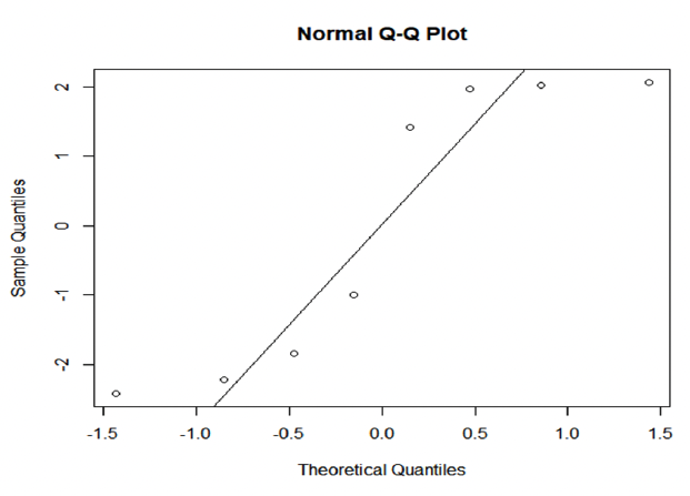
Gannet

A normal Q-Q plot for large gulls with sample quantities on the y axis ranging from -2.5 to 2.1and theoretical quantiles in the x axis ranging from -1.6 to 1.6. The line of best fit starts from -0.8 theoretical quantiles and extends up to 0.65 — Figure IV.9 Q-Q line plot of the LM of flight height of large gulls against the distance to the nearest turbine.

Comparing flight height in different area with and without WGTs

Core species (large gulls, kittiwake, fulmar, gannet)

Wilcoxon rank sum test with continuity correction

data: corspec$BirdZ_SeaL by corspec$area

W = 56813, p-value = 0.000000000000001543

alternative hypothesis: true location shift is not equal to 0

95 percent confidence interval:

-3.980004 -1.520024

sample estimates:

difference in location

-2.719962

Area1 Mean height seaL= 11.32 m s.d= 26.61

Area2 Mean height seaL 20.03 = s.d= 33.73

Kittiwake

Wilcoxon rank sum test with continuity correction

data: kittiwake$BirdZ_SeaL by kittiwake$area

W = 34715, p-value = 0.000001006

alternative hypothesis: true location shift is not equal to 0

95 percent confidence interval:

-3.3299740 -0.7600427

sample estimates:

difference in location

-1.839956

Area1 Mean height seaL= 12.49 s.d= 24.87

Area2 Mean height seaL= 17.84 s.d= 30.83

Fulmar

Wilcoxon rank sum test with continuity correction

data: fulmar$BirdZ_SeaL by fulmar$area

W = 1237.5, p-value = 0.05343

alternative hypothesis: true location shift is not equal to 0

95 percent confidence interval:

-0.78999810008 0.00003286683

sample estimates:

difference in location

-0.299965

Area1 Mean height seaL= 1.72 s.d= 5.34

Area2 Mean height seaL= 3.53 s.d= 7.89

Gannet

Wilcoxon rank sum test with continuity correction

data: gannet$BirdZ_SeaL by gannet$area

W = 181.5, p-value = 0.004449

alternative hypothesis: true location shift is not equal to 0

95 percent confidence interval:

-9.6579730 -0.4699419

sample estimates:

difference in location

-5.960084

Area1 Mean height seaL= 2.45 s.d= 2.96

Area2 Mean height seaL= 12.89 s.d= 18.44

Gull

Wilcoxon rank sum test with continuity correction

data: gull$BirdZ_SeaL by gull$area

W = 154, p-value = 0.8703

alternative hypothesis: true location shift is not equal to 0

95 percent confidence interval:

-47.63005 61.76006

sample estimates:

difference in location

4.263862

Area1 Mean height seaL= 81.92 s.d= 72.49

Area2 Mean height seaL= 72.40 s.d= 48.05

Comparing flight height in relation to distance to nearest WGT

Core species (large gulls, kittiwake, fulmar, gannet)

Linear mixed model fit by REML. t-tests use Satterthwaite's method ['lmerModLmerTest']

Formula: ((BirdZ_SeaL^lambda - 1)/lambda) ~ Turbine_Distance_M_scaled * (1 | CommonName) + (1 | month)

Data: area1

REML criterion at convergence: 898.8

Scaled residuals:

Min 1Q Median 3Q Max

-2.61097 -0.79216 -0.00487 0.79954 2.05542

Random effects:

Groups Name Variance Std.Dev.

CommonName (Intercept) 1.2132 1.1015

month (Intercept) 0.3051 0.5523

Residual 0.9589 0.9792

Number of obs: 315, groups: CommonName, 5; month, 2

Fixed effects:

Estimate Std. Error df t value Pr(>|t|)

(Intercept) 0.9688 0.6506 4.1117 1.489 0.209

Turbine_Distance_M_scaled 0.2832 0.3564 310.0732 0.795 0.427

Correlation of Fixed Effects:

(Intr)

Trbn_Dst_M_ -0.108

Kittiwake

Generalized linear mixed model fit by maximum likelihood (Laplace Approximation) ['glmerMod']

Family: inverse.gaussian ( 1/mu^2 )

Formula: BirdZ_SeaL_sqrt ~ Turbine_Distance_M_scaled + (1 | month)

Data: kittiwake

AIC BIC logLik deviance df.resid

763.8 777.4 -377.9 755.8 216

Scaled residuals:

Min 1Q Median 3Q Max

-0.9350 -0.7283 -0.4153 0.4196 4.4823

Random effects:

Groups Name Variance Std.Dev.

month (Intercept) 0.003769 0.06139

Residual 0.294173 0.54238

Number of obs: 220, groups: month, 2

Fixed effects:

Estimate Std. Error t value Pr(>|z|)

(Intercept) 0.16771 0.07766 2.160 0.0308 *

Turbine_Distance_M_scaled -0.05798 0.09470 -0.612 0.5404

Signif. codes: 0 '***' 0.001 '**' 0.01 '*' 0.05 '.' 0.1 ' ' 1

Correlation of Fixed Effects:

(Intr)

Trbn_Dst_M_ -0.261

Fulmar

Linear mixed model fit by REML. t-tests use Satterthwaite's method ['lmerModLmerTest']

Formula: BirdZ_SeaL ~ Turbine_Distance_M_scaled + (1 | month)

Data: fulmar

REML criterion at convergence: 423.7

Scaled residuals:

Min 1Q Median 3Q Max

-0.6277 -0.2298 -0.1253 0.0502 7.8833

Random effects:

Groups Name Variance Std.Dev.

month (Intercept) 2.676 1.636

Residual 27.290 5.224

Number of obs: 70, groups: month, 2

Fixed effects:

Estimate Std. Error df t value Pr(>|t|)

(Intercept) 2.761 1.536 1.708 1.798 0.235

Turbine_Distance_M_scaled -3.841 4.525 67.554 -0.849 0.399

Correlation of Fixed Effects:

(Intr)

Trbn_Dst_M_ -0.498

Gannet

Linear mixed model fit by REML. t-tests use Satterthwaite's method ['lmerModLmerTest']

Formula: BirdZ_SeaL ~ Turbine_Distance_M_scaled + (1 | month)

Data: gannet

REML criterion at convergence: 69.3

Scaled residuals:

Min 1Q Median 3Q Max

-1.3060 -0.7526 -0.3054 0.8807 1.5152

Random effects:

Groups Name Variance Std.Dev.

month (Intercept) 1.431 1.196

Residual 4.304 2.075

Number of obs: 17, groups: month, 2

Fixed effects:

Estimate Std. Error df t value Pr(>|t|)

(Intercept) 0.3622 1.1329 1.0882 0.320 0.799591

Turbine_Distance_M_scaled 5.7669 1.3873 14.5092 4.157 0.000901 ***

Signif. codes: 0 '***' 0.001 '**' 0.01 '*' 0.05 '.' 0.1 ' ' 1

Correlation of Fixed Effects:

(Intr)

Trbn_Dst_M_ -0.466

Gull (only July)

Call:

lm(formula = gull$BirdZ_SeaL_sqrt ~ gull$Turbine_Distance_M_scaled)

Residuals:

Min 1Q Median 3Q Max

-2.4172 -1.9338 0.2128 1.9764 2.0664

Coefficients:

Estimate Std. Error t value Pr(>|t|)

(Intercept) 12.574 1.187 10.591 0.0000417 ***

gull$Turbine_Distance_M_scaled -33.238 6.217 -5.346 0.00175 **

---

Signif. codes: 0 '***' 0.001 '**' 0.01 '*' 0.05 '.' 0.1 ' ' 1

Residual standard error: 2.211 on 6 degrees of freedom

Multiple R-squared: 0.8265, Adjusted R-squared: 0.7976

F-statistic: 28.58 on 1 and 6 DF, p-value: 0.001751

R Script for Linear Mixed Modelling and Distance to Turbine Histograms

#### R code for Models and Distance to Turbines (m) ####

#### Created by Alexandra McCubbin and Beate Zein for APEM Ltd

#### Section below created by Beate Zein for APEM Ltd

rm(list = ls())

#### Install packages... ####

library(nlme)

library(lme4)

library(tidyverse)

library(ggeffects)

library(stargazer)

library(arsenal)

#set working directory and select data

path_out = "C:"

options(scipen = 999) # prevents small/large numbers being shown in e format

#June data

setwd("C:/")

testfiles <-list.files("C:/") ### assign files in the directory as 'testfiles'

testfiles

#### Read in Data for each site ####

June_Beatrice <- read.csv(paste0(getwd(), "/", testfiles[1]))

June_MorayEast <- read.csv(paste0(getwd(), "/", testfiles[2]))

June_Outwith <- read.csv(paste0(getwd(), "/", testfiles[3]))

June_Survey2 <- read.csv(paste0(getwd(), "/", testfiles[4]))

#### Add Location Column ####

June_Beatrice$Location="Beatrice"

June_MorayEast$Location="Moray East"

June_Outwith$Location="S1Outwith"

June_Survey2$Location="Survey2"

#### Combine into one DataFrame ####

CombinedJune <-rbind(June_Beatrice, June_MorayEast, June_Outwith, June_Survey2)

#### JULY Set WD####

setwd("C:/")

testfilesJul <-list.files("C:/") ### assign files in the directory as 'testfiles'

testfilesJul

#### Read in Data for each site ####

July_Beatrice <- read.csv(paste0(getwd(), "/", testfilesJul[1]))

July_MorayEast <- read.csv(paste0(getwd(), "/", testfilesJul[2]))

July_Outwith <- read.csv(paste0(getwd(), "/", testfilesJul[3]))

July_Survey2 <- read.csv(paste0(getwd(), "/", testfilesJul[4]))

#### Add Location Column ####

July_Beatrice$Location="Beatrice"

July_MorayEast$Location="Moray East"

July_Outwith$Location="S1Outwith"

July_Survey2$Location="Survey2"

#### Combine into one DataFrame ####

CombinedJuly <-rbind(July_Beatrice, July_MorayEast, July_Outwith, July_Survey2)

rm(July_Beatrice,July_MorayEast, July_Outwith, July_Survey2,June_Beatrice,June_MorayEast, June_Outwith, June_Survey2)

#### Drop Extra Column From July ####

CombinedJuly <- CombinedJuly[-c(30)]

#add month running number

CombinedJune$month<-6

CombinedJuly$month<-7

colnames(CombinedJuly)

colnames(CombinedJune) ### check June and July Column Names Match

#### Combine All Data ####

JuneJulyCombine <- rbind(CombinedJune, CombinedJuly)

#### Summaries ####

summary(CombinedJuly)

summary(CombinedJune)

summary(JuneJulyCombine)

#add survey area 1 and 2

JuneJulyCombine$area<-1

JuneJulyCombine$area[JuneJulyCombine$Location=="Survey2"]<- 2

#remove NA in height data

JuneJulyCombine<-JuneJulyCombine[!is.na(JuneJulyCombine$BirdZ_SeaL),]

#split up by species

unique(JuneJulyCombine$CommonName)

fulmar<-JuneJulyCombine[JuneJulyCombine$CommonName == "Fulmar",]

kittiwake<-JuneJulyCombine[JuneJulyCombine$CommonName == "Kittiwake",]

gannet<-JuneJulyCombine[JuneJulyCombine$CommonName == "Gannet",]

gull<-JuneJulyCombine[JuneJulyCombine$CommonName == "Herring Gull"|JuneJulyCombine$CommonName == "Great Black-backed Gull",]

#select core species of interest

corspec<-rbind(fulmar,kittiwake,gannet,gull)

#compare flight height of different study sides

#Mann Whithey U test /Wilcoxon rank sum test

#not measured randomly, left skewed distribution, none equal variance

#non-parametric

#Ho median if flight height is the same in the two areas

#all core species

var(corspec$BirdZ_SeaL[corspec$area=="1"])

var(corspec$BirdZ_SeaL[corspec$area=="2"])

#none equal variances

hist(corspec$BirdZ_SeaL[corspec$area=="1"],breaks=50)

boxplot(corspec$BirdZ_SeaL~corspec$area)

mean(corspec$BirdZ_SeaL[corspec$area=="1"])

sd(corspec$BirdZ_SeaL[corspec$area=="1"])

sd(corspec$BirdZ_SeaL[corspec$area=="2"])

mean(corspec$BirdZ_SeaL[corspec$area=="2"])

#test

wilcox.test(corspec$BirdZ_SeaL~corspec$area,mu=0,alt="two.sided",conf.int=T,conf.level=0.95,paired=FALSE,exact=F,correct=T) # where y1 and y2 are numeric

#kittiwake

var(kittiwake$BirdZ_SeaL[kittiwake$area=="1"])

var(kittiwake$BirdZ_SeaL[kittiwake$area=="2"])

#none equal variances

hist(kittiwake$BirdZ_SeaL[kittiwake$area=="1"],breaks=50)

hist(kittiwake$BirdZ_SeaL[kittiwake$area=="2"],breaks=50)

boxplot(kittiwake$BirdZ_SeaL~kittiwake$area)

mean(kittiwake$BirdZ_SeaL[kittiwake$area=="1"])

mean(kittiwake$BirdZ_SeaL[kittiwake$area=="2"])

sd(kittiwake$BirdZ_SeaL[kittiwake$area=="1"])

sd(kittiwake$BirdZ_SeaL[kittiwake$area=="2"])

#test

wilcox.test(kittiwake$BirdZ_SeaL~kittiwake$area,mu=0,alt="two.sided",conf.int=T,conf.level=0.95,paired=FALSE,exact=F,correct=T) # where y1 and y2 are numeric

#fulmar

var(fulmar$BirdZ_SeaL[fulmar$area=="1"])

var(fulmar$BirdZ_SeaL[fulmar$area=="2"])

#none equal variances

hist(fulmar$BirdZ_SeaL[fulmar$area=="1"],breaks=50)

hist(fulmar$BirdZ_SeaL[fulmar$area=="2"],breaks=50)

boxplot(fulmar$BirdZ_SeaL~fulmar$area)

mean(fulmar$BirdZ_SeaL[fulmar$area=="1"])

mean(fulmar$BirdZ_SeaL[fulmar$area=="2"])

sd(fulmar$BirdZ_SeaL[fulmar$area=="1"])

sd(fulmar$BirdZ_SeaL[fulmar$area=="2"])

#test

wilcox.test(fulmar$BirdZ_SeaL~fulmar$area,mu=0,alt="two.sided",conf.int=T,conf.level=0.95,paired=FALSE,exact=F,correct=T) # where y1 and y2 are numeric

#gannet

var(gannet$BirdZ_SeaL[gannet$area=="1"])

var(gannet$BirdZ_SeaL[gannet$area=="2"])

#none equal variances

hist(kittiwake$BirdZ_SeaL[kittiwake$area=="1"],breaks=50)

hist(kittiwake$BirdZ_SeaL[kittiwake$area=="2"],breaks=50)

boxplot(gannet$BirdZ_SeaL~gannet$area)

mean(gannet$BirdZ_SeaL[gannet$area=="1"])

mean(gannet$BirdZ_SeaL[gannet$area=="2"])

sd(gannet$BirdZ_SeaL[gannet$area=="1"])

sd(gannet$BirdZ_SeaL[gannet$area=="2"])

#test

wilcox.test(gannet$BirdZ_SeaL~gannet$area,mu=0,alt="two.sided",conf.int=T,conf.level=0.95,paired=FALSE,exact=F,correct=T) # where y1 and y2 are numeric

#gull

var(gull$BirdZ_SeaL[gull$area=="1"])

var(gull$BirdZ_SeaL[gull$area=="2"])

#none equal variances

hist(kittiwake$BirdZ_SeaL[kittiwake$area=="1"],breaks=50)

hist(kittiwake$BirdZ_SeaL[kittiwake$area=="2"],breaks=50)

boxplot(gull$BirdZ_SeaL~gull$area)

mean(gull$BirdZ_SeaL[gull$area=="1"])

mean(gull$BirdZ_SeaL[gull$area=="2"])

sd(gull$BirdZ_SeaL[gull$area=="1"])

sd(gull$BirdZ_SeaL[gull$area=="2"])

#test

wilcox.test(gull$BirdZ_SeaL~gull$area,mu=0,alt="two.sided",conf.int=T,conf.level=0.95,paired=FALSE,exact=F,correct=T) # where y1 and y2 are numeric

#make violin plot for all core species

corspec$area<-as.factor(corspec$area)

library(ggplot2)

GeomSplitViolin <- ggproto("GeomSplitViolin", GeomViolin,

draw_group = function(self, data, ..., draw_quantiles = NULL) {

data <- transform(data, xminv = x - violinwidth * (x - xmin), xmaxv = x + violinwidth * (xmax - x))

grp <- data[1, "group"]

newdata <- plyr::arrange(transform(data, x = if (grp %% 2 == 1) xminv else xmaxv), if (grp %% 2 == 1) y else -y)

newdata <- rbind(newdata[1, ], newdata, newdata[nrow(newdata), ], newdata[1, ])

newdata[c(1, nrow(newdata) - 1, nrow(newdata)), "x"] <- round(newdata[1, "x"])

if (length(draw_quantiles) > 0 & !scales::zero_range(range(data$y))) {

stopifnot(all(draw_quantiles >= 0), all(draw_quantiles <=

1))

quantiles <- ggplot2:::create_quantile_segment_frame(data, draw_quantiles)

aesthetics <- data[rep(1, nrow(quantiles)), setdiff(names(data), c("x", "y")), drop = FALSE]

aesthetics$alpha <- rep(1, nrow(quantiles))

both <- cbind(quantiles, aesthetics)

quantile_grob <- GeomPath$draw_panel(both, ...)

ggplot2:::ggname("geom_split_violin", grid::grobTree(GeomPolygon$draw_panel(newdata, ...), quantile_grob))

}

else {

ggplot2:::ggname("geom_split_violin", GeomPolygon$draw_panel(newdata, ...))

}

})

geom_split_violin <- function(mapping = NULL, data = NULL, stat = "ydensity", position = "identity", ...,

draw_quantiles = NULL, trim = TRUE, scale = "area", na.rm = FALSE,

show.legend = NA, inherit.aes = TRUE) {

layer(data = data, mapping = mapping, stat = stat, geom = GeomSplitViolin,

position = position, show.legend = show.legend, inherit.aes = inherit.aes,

params = list(trim = trim, scale = scale, draw_quantiles = draw_quantiles, na.rm = na.rm, ...))

}

#scale and log data for check

corspec$BirdZ_SeaL_scales<-scale(corspec$BirdZ_SeaL, center = TRUE, scale = TRUE)

hist(corspec$BirdZ_SeaL_scales)

corspec$BirdZ_SeaL_log<-log(corspec$BirdZ_SeaL)

#rename Great Black-backed gull and herring gull

corspec_plot<-corspec

corspec_plot$CommonName<-gsub("Great Black-backed Gull" , "Large Gull",corspec_plot$CommonName)

corspec_plot$CommonName<-gsub("Herring Gull" , "Large Gull",corspec_plot$CommonName)

#split data by scale of distance

fulgan<-corspec_plot[corspec_plot$CommonName=="Fulmar"|corspec_plot$CommonName=="Gannet",]

kitgul<-corspec_plot[corspec_plot$CommonName=="Kittiwake"|corspec_plot$CommonName=="Large Gull",]

#make the plots

library(cowplot)

#June

#no fulmar and gannet in june

kitgul_June<-kitgul[kitgul$month==6,]

plot2<-ggplot(kitgul_June, aes(x=CommonName, y=BirdZ_SeaL, fill = area)) + geom_split_violin()+

labs(y = "height above sealevel [m]") +

theme(axis.title.x = element_blank(),axis.text=element_text(size=14),

axis.title=element_text(size=14,face="bold"),axis.text.x = element_text(angle = 15, hjust=1))

ggsave("cor_species_flightheight_JUNE_seperatescale.png",path = "C:/", device='png', dpi=300,plot2)

#July

fulgan_July<-fulgan[fulgan$month==7,]

kitgul_July<-kitgul[kitgul$month==7,]

plot1<-ggplot(fulgan_July, aes(x=CommonName, y=BirdZ_SeaL, fill = area)) + geom_split_violin()+

labs(y = "height above sealevel [m]") +

theme(axis.title.x = element_blank(),legend.position="none",axis.text=element_text(size=14),

axis.title=element_text(size=14,face="bold"),axis.text.x = element_text(angle = 15, hjust=1))

plot2<-ggplot(kitgul_July, aes(x=CommonName, y=BirdZ_SeaL, fill = area)) + geom_split_violin()+

theme(axis.title.x = element_blank(),axis.title.y = element_blank(),axis.text=element_text(size=14),

axis.title=element_text(size=14,face="bold"),axis.text.x = element_text(angle = 15, hjust=1))

plot_grid(plot1, plot2, labels = "AUTO")

p<-plot_grid(plot1, plot2, labels = "AUTO")

ggsave("cor_species_flightheight_JULY_seperatescale.png",path = "C:/", device='png', dpi=300,p)

# analyse flight height in relation to distance to turbines

#check different distributions

library(fitdistrplus)

fw <- fitdist(corspec$BirdZ_SeaL, "weibull")

fg <- fitdist(corspec$BirdZ_SeaL, "gamma")

fln <- fitdist(corspec$BirdZ_SeaL, "lnorm")

fn <- fitdist(corspec$BirdZ_SeaL, "norm")

fpoi <- fitdist(corspec$BirdZ_SeaL, "pois")

### plot it

par(mfrow = c(2, 2))

plot.legend <- c("Weibull", "lognormal", "gamma", "normal")

denscomp(list(fw, fln, fg, fn), legendtext = plot.legend)

qqcomp(list(fw, fln, fg, fn), legendtext = plot.legend)

cdfcomp(list(fw, fln, fg, fn), legendtext = plot.legend)

ppcomp(list(fw, fln, fg, fn), legendtext = plot.legend)

###

#models

library(lme4)

library(car)

corspec$CommonName<-as.factor(corspec$CommonName)

corspec$Turbine_Distance_M_scaled <- scale(corspec$Turbine_Distance_M, center = FALSE, scale = TRUE)

area1<-corspec[corspec$area == 1,]

area2<-corspec[corspec$area == 2,]

#area 1 test for normal and others

hist(area1$BirdZ_SeaL,breaks = 100)

area1$BirdZ_SeaL_log<-log(area1$BirdZ_SeaL)

fw <- fitdist(area1$BirdZ_SeaL, "weibull")

fg <- fitdist(area1$BirdZ_SeaL, "gamma")

fln <- fitdist(area1$BirdZ_SeaL, "lnorm")

fn <- fitdist(area1$BirdZ_SeaL, "norm")

fpoi <- fitdist(area1$BirdZ_SeaL, "pois")

### plot it

par(mfrow = c(2, 2))

plot.legend <- c("Weibull", "lognormal", "gamma", "normal")

denscomp(list(fw, fln, fg, fn), legendtext = plot.legend)

qqcomp(list(fw, fln, fg, fn), legendtext = plot.legend)

cdfcomp(list(fw, fln, fg, fn), legendtext = plot.legend)

ppcomp(list(fw, fln, fg, fn), legendtext = plot.legend)

plot(area1$Turbine_Distance_M,area1$BirdZ_SeaL)

#kittiwake

hist(kittiwake$BirdZ_SeaL,breaks = 50)

hist(kittiwake$Turbine_Distance_M,breaks = 50)

hist(kittiwake$Turbine_Distance_M_log,breaks = 50)

hist(sqrt(kittiwake$Turbine_Distance_M),breaks = 50)

#Fulmar

hist(fulmar$BirdZ_SeaL,breaks = 50)

hist(fulmar$Turbine_Distance_M,breaks = 50)

#gannet

hist(gannet$BirdZ_SeaL,breaks = 50)

hist(gannet$Turbine_Distance_M,breaks = 50)

#guills

hist(gull$BirdZ_SeaL,breaks = 50)

hist(gull$Turbine_Distance_M,breaks = 50)

#Fulamr

plot(fulmar$Turbine_Distance_M_log,log(fulmar$BirdZ_SeaL))

plot(fulmar$Turbine_Distance_M,fulmar$BirdZ_SeaL)

#load the libraries

library(glmm)

library(lme4)

JuneJulyCombine$month<-as.factor(JuneJulyCombine$month)

kittiwake$month<-as.factor(kittiwake$month)

kittiwake$Turbine_Distance_M<-as.integer(kittiwake$Turbine_Distance_M)

kittiwake$BirdZ_SeaL<-as.integer(kittiwake$BirdZ_SeaL)

kittiwake$BirdZ_SeaL_log<-log(kittiwake$BirdZ_SeaL)

corspec$Turbine_Distance_M_scaled_log<-log(corspec$Turbine_Distance_M_scaled)

corspec$BirdZ_SeaL_log<-log(corspec$BirdZ_SeaL)

corspec$BirdZ_SeaL_sqrt<-sqrt(corspec$BirdZ_SeaL)

area1<-corspec[corspec$area == 1,]

##### Models ####

# Core species in area 1

hist(area1$BirdZ_SeaL,breaks = 50)

#find optimal lambda for Box-Cox transformation

bc <- boxcox(area1$BirdZ_SeaL ~ area1$Turbine_Distance_M_scaled)

lambda <- bc$x[which.max(bc$y)]

lambda

library(lmerTest)

#fit new linear regression model using the Box-Cox transformation

mixedmodelarea1 <- lmer(((BirdZ_SeaL^lambda-1)/lambda) ~ Turbine_Distance_M_scaled * (1|CommonName) + (1|month), data = area1)

summary(mixedmodelarea1)

plot(mixedmodelarea1,xlab="Fitted values", ylab="Residuals", which = 2)

qqnorm(resid(mixedmodelarea1))

qqline(resid(mixedmodelarea1))

# #### Turbine Distance raw plot ####

testplot <- ggplot (area1, aes(x = Turbine_Distance_M_scaled, y = BirdZ_SeaL,color=CommonName)) +

geom_point()+

labs(x= "Distance to WTG [m]", y = "height above sealevel [m]") +

theme(axis.text=element_text(size=14),axis.title=element_text(size=14,face="bold"))+

geom_smooth (method="lm")

ggsave("cor_species_flightheight_distanceturbine.png",path = "C:/Users/b.zein/OneDrive - Apem Limited/P5794/LiDAR Mixed Model/outputs_new/", device='png', dpi=300,testplot)

#take common names from area 1 only for distance to turbine as no turbines in area2

fulmar<-area1[area1$CommonName == "Fulmar",]

kittiwake<-area1[area1$CommonName == "Kittiwake",]

gannet<-area1[area1$CommonName == "Gannet",]

gull<-area1[area1$CommonName == "Herring Gull"|area1$CommonName == "Great Black-backed Gull",]

hist(area1$Turbine_Distance_M, breaks = 109)

#kittiwake

hist(kittiwake$BirdZ_SeaL,breaks=500)

length(kittiwake$Bird_No)

#glmm

require(lme4)

combo <- glmer(BirdZ_SeaL_sqrt ~ Turbine_Distance_M_scaled + (1|month) , data = kittiwake,family=inverse.gaussian(link = "1/mu^2"))

summary(combo )

plot(combo , which = 2)

qqnorm(resid(combo ))

qqline(resid(combo ))

#fulmar

hist(fulmar$BirdZ_SeaL_sqrt,breaks=66)

#LM

combof <-lm(BirdZ_SeaL ~ Turbine_Distance_M_scaled, data = fulmar)

summary(combof )

plot(combof , which = 2)

qqnorm(resid(combof ))

qqline(resid(combof ))

#gannet

hist(gannet$BirdZ_SeaL,breaks=500)

#LM

combog <-lm(BirdZ_SeaL~ Turbine_Distance_M_scaled, data = gannet)

summary(combog )

plot(combog , which = 2)

qqnorm(resid(combog ))

qqline(resid(combog ))

#gull #only sample 1 in june and 8 in july

#remove June for modelling

gull<-gull[-1,]

hist(gull$BirdZ_SeaL_sqrt,breaks=500)

#LM

combog <-lm(BirdZ_SeaL_sqrt ~ Turbine_Distance_M_scaled, data = gull)

summary(combog )

plot(combog , which = 2)

qqnorm(resid(combog ))

qqline(resid(combog ))

#### Section below created by created by Alexandra McCubbin for APEM Ltd

### Histogram distance to WTG for each species

#### Dist to Turbine by spp June ####

setwd("C:/ ")

colnames(CombinedJune)

unique(CombinedJune$CommonName)

JuneFulmar <- subset(CombinedJune, CommonName =="Fulmar")

JuneKittiwake <- subset(CombinedJune, CommonName=="Kittiwake")

JuneGuillemot <- subset(CombinedJune, CommonName == "Guillemot")

JuneRazorbill <- subset(CombinedJune, CommonName == "Razorbill")

JuneGuillRaz <- subset(CombinedJune, CommonName == "Guillemot/Razorbill")

JuneGannet <- subset(CombinedJune, CommonName == "Gannet")

JuneSkua <- subset(CombinedJune, CommonName == "Great Skua")

JuneHerrGu <- subset(CombinedJune, CommonName == "Herring Gull")

JuneGBbg <- subset(CombinedJune, CommonName == "Great Black-backed Gull")

JuneAukSh <- subset(CombinedJune, CommonName == "Auk/Shearwater species")

JuneAukspp <- subset(CombinedJune, CommonName == "Auk species")

ggplot(JuneFulmar, aes(x=Turbine_Distance_M)) +

geom_histogram(fill='#317FA0', color="black", binwidth = 5000)+

#facet_grid(alltog2$Survey)+

labs(x = "Fulmar Distance to Turbine (m)", y = "Frequency")+

theme_classic()+

theme(axis.text.x = element_text(angle = 30, hjust = 1))+

theme(text = element_text(size=16))

filenameFulmarJune<-"June_Fulmar_Hist.png"

ggsave(filenameFulmarJune, width = 11, height =7)

ggplot(JuneKittiwake, aes(x=Turbine_Distance_M)) +

geom_histogram(fill='#317FA0', color="black", binwidth = 5000)+

#facet_grid(alltog2$Survey)+

labs(x = "Kittiwake Distance to Turbine (m)", y = "Frequency")+

theme_classic()+

theme(axis.text.x = element_text(angle = 30, hjust = 1))+

theme(text = element_text(size=16))

filenameKittiwakeJune<-"June_Kittiwake_Hist.png"

ggsave(filenameKittiwakeJune, width = 11, height =7)

ggplot(JuneGuillemot, aes(x=Turbine_Distance_M)) +

geom_histogram(fill='#317FA0', color="black", binwidth = 5000)+

#facet_grid(alltog2$Survey)+

labs(x = "Guillemot Distance to Turbine (m)", y = "Frequency")+

theme_classic()+

theme(axis.text.x = element_text(angle = 30, hjust = 1))+

theme(text = element_text(size=16))

filenameGuillemotJune<-"June_Guillemot_Hist.png"

ggsave(filenameGuillemotJune, width = 11, height =7)

ggplot(JuneRazorbill, aes(x=Turbine_Distance_M)) +

geom_histogram(fill='#317FA0', color="black", binwidth = 5000)+

#facet_grid(alltog2$Survey)+

labs(x = "Razorbill Distance to Turbine (m)", y = "Frequency")+

theme_classic()+

theme(axis.text.x = element_text(angle = 30, hjust = 1))+

theme(text = element_text(size=16))

filenameRazorbillJune<-"June_Razorbill_Hist.png"

ggsave(filenameRazorbillJune, width =11, height =7)

ggplot(JuneGuillRaz, aes(x=Turbine_Distance_M)) +

geom_histogram(fill='#317FA0', color="black", binwidth = 5000)+

#facet_grid(alltog2$Survey)+

labs(x = "Guillemont/Razorbill Distance to Turbine (m)", y = "Frequency")+

theme_classic()+

theme(axis.text.x = element_text(angle = 30, hjust = 1))+

theme(text = element_text(size=16))

filenameGuillRazJune<-"June_GuillRaz_Hist.png"

ggsave(filenameGuillRazJune, width = 11, height =7)

ggplot(JuneGannet, aes(x=Turbine_Distance_M)) +

geom_histogram(fill='#317FA0', color="black", binwidth = 5000)+

#facet_grid(alltog2$Survey)+

labs(x = "Gannet Distance to Turbine (m)", y = "Frequency")+

theme_classic()+

theme(axis.text.x = element_text(angle = 30, hjust = 1))+

theme(text = element_text(size=16))

filenameGannetJune<-"June_Gannet_Hist.png"

ggsave(filenameGannetJune, width = 11, height =7)

ggplot(JuneSkua, aes(x=Turbine_Distance_M)) +

geom_histogram(fill='#317FA0', color="black", binwidth = 5000)+

#facet_grid(alltog2$Survey)+

labs(x = "Great Skua Distance to Turbine (m)", y = "Frequency")+

theme_classic()+

theme(axis.text.x = element_text(angle = 30, hjust = 1))+

theme(text = element_text(size=16))

filenameSkuaJune<-"June_Skua_Hist.png"

ggsave(filenameSkuaJune, width = 11, height =7)

ggplot(JuneHerrGu, aes(x=Turbine_Distance_M)) +

geom_histogram(fill='#317FA0', color="black", binwidth = 5000)+

#facet_grid(alltog2$Survey)+

labs(x = "Herring Gull Distance to Turbine (m)", y = "Frequency")+

theme_classic()+

theme(axis.text.x = element_text(angle = 30, hjust = 1))+

theme(text = element_text(size=16))

filenameHerrGuJune<-"June_HerrGu_Hist.png"

ggsave(filenameHerrGuJune, width = 11, height =7)

ggplot(JuneGBbg, aes(x=Turbine_Distance_M)) +

geom_histogram(fill='#317FA0', color="black", binwidth = 5000)+

#facet_grid(alltog2$Survey)+

labs(x = "Great Black-backed Gull Distance to Turbine (m)", y = "Frequency")+

theme_classic()+

theme(axis.text.x = element_text(angle = 30, hjust = 1))+

theme(text = element_text(size=16))

filenameGBbgJune<-"June_GBbg_Hist.png"

ggsave(filenameGBbgJune, width = 11, height =7)

ggplot(JuneAukSh, aes(x=Turbine_Distance_M)) +

geom_histogram(fill='#317FA0', color="black", binwidth = 5000)+

#facet_grid(alltog2$Survey)+

labs(x = "Auk/shearwater Distance to Turbine (m)", y = "Frequency")+

theme_classic()+

theme(axis.text.x = element_text(angle = 30, hjust = 1))+

theme(text = element_text(size=16))

filenameAukShJune<-"June_AukSh_Hist.png"

ggsave(filenameAukShJune, width = 11, height =7)

ggplot(JuneAukspp, aes(x=Turbine_Distance_M)) +

geom_histogram(fill='#317FA0', color="black", binwidth = 5000)+

#facet_grid(alltog2$Survey)+

labs(x = "Auk Species Distance to Turbine (m)", y = "Frequency")+

theme_classic()+

theme(axis.text.x = element_text(angle = 30, hjust = 1))+

theme(text = element_text(size=16))

filenameAuksppJune<-"June_Aukspp_Hist.png"

ggsave(filenameAuksppJune, width = 11, height =7)

#### Dist to Turbine by spp July ####

colnames(CombinedJuly)

unique(CombinedJuly$CommonName)

setwd("C:/ ")

JulyFulmar <- subset(CombinedJuly, CommonName =="Fulmar")

JulyGannet <- subset(CombinedJuly, CommonName == "Gannet")

JulySkua <- subset(CombinedJuly, CommonName == "Great Skua")

JulyGuillemot <- subset(CombinedJuly, CommonName == "Guillemot")

JulyHerrGu <- subset(CombinedJuly, CommonName == "Herring Gull")

JulyKittiwake <- subset(CombinedJuly, CommonName=="Kittiwake")

JulyGBbg <- subset(CombinedJuly, CommonName == "Great Black-backed Gull")

JulyGuillRaz <- subset(CombinedJuly, CommonName == "Guillemot/Razorbill")

JulyPuffin <- subset(CombinedJuly, CommonName == "Puffin")

JulyUnIDBirSpp <- subset(CombinedJuly, CommonName == "Unidentified Bird species")

JulyManx <- subset(CombinedJuly, CommonName == "Manx Shearwater")

ggplot(JulyFulmar, aes(x=Turbine_Distance_M)) +

geom_histogram(fill='#317FA0', color="black", binwidth = 5000)+

#facet_grid(alltog2$Survey)+

labs(x = "Fulmar Distance to Turbine (m)", y = "Frequency")+

theme_classic()+

theme(axis.text.x = element_text(angle = 30, hjust = 1))+

theme(text = element_text(size=16))

filenameFulmarJuly<-"July_Fulmar_Hist.png"

ggsave(filenameFulmarJuly, width = 11, height =7)

ggplot(JulyGannet, aes(x=Turbine_Distance_M)) +

geom_histogram(fill='#317FA0', color="black", binwidth = 5000)+

#facet_grid(alltog2$Survey)+

labs(x = "Gannet Distance to Turbine (m)", y = "Frequency")+

theme_classic()+

theme(axis.text.x = element_text(angle = 30, hjust = 1))+

theme(text = element_text(size=16))

filenameGannetJuly<-"July_Gannet_Hist.png"

ggsave(filenameGannetJuly, width = 11, height =7)

ggplot(JulySkua, aes(x=Turbine_Distance_M)) +

geom_histogram(fill='#317FA0', color="black", binwidth = 1000)+

#facet_grid(alltog2$Survey)+

labs(x = "Great Skua Distance to Turbine (m)", y = "Frequency")+

theme_classic()+

theme(axis.text.x = element_text(angle = 30, hjust = 1))+

theme(text = element_text(size=16))

filenameSkuaJuly<-"July_Skua_Hist.png"

ggsave(filenameSkuaJuly, width = 11, height =7)

ggplot(JulyGuillemot, aes(x=Turbine_Distance_M)) +

geom_histogram(fill='#317FA0', color="black", binwidth = 5000)+

#facet_grid(alltog2$Survey)+

labs(x = "Guillemot Distance to Turbine (m)", y = "Frequency")+

theme_classic()+

theme(axis.text.x = element_text(angle = 30, hjust = 1))+

theme(text = element_text(size=16))

filenameGuillemotJuly<-"July_Guillemot_Hist.png"

ggsave(filenameGuillemotJuly, width = 11, height =7)

ggplot(JulyHerrGu, aes(x=Turbine_Distance_M)) +

geom_histogram(fill='#317FA0', color="black", binwidth = 5000)+

#facet_grid(alltog2$Survey)+

labs(x = "Herring Gull Distance to Turbine (m)", y = "Frequency")+

theme_classic()+

theme(axis.text.x = element_text(angle = 30, hjust = 1))+

theme(text = element_text(size=16))

filenameHerrGuJuly<-"July_HerrGu_Hist.png"

ggsave(filenameHerrGuJuly, width = 11, height =7)

ggplot(JulyKittiwake, aes(x=Turbine_Distance_M)) +

geom_histogram(fill='#317FA0', color="black", binwidth = 5000)+

#facet_grid(alltog2$Survey)+

labs(x = "Kittiwake Distance to Turbine (m)", y = "Frequency")+

theme_classic()+

theme(axis.text.x = element_text(angle = 30, hjust = 1))+

theme(text = element_text(size=16))

filenameKittiwakeJuly<-"July_Kittiwake_Hist.png"

ggsave(filenameKittiwakeJuly, width = 11, height =7)

ggplot(JulyGBbg, aes(x=Turbine_Distance_M)) +

geom_histogram(fill='#317FA0', color="black", binwidth = 5000)+

#facet_grid(alltog2$Survey)+

labs(x = "Great Black-backed Gull Distance to Turbine (m)", y = "Frequency")+

theme_classic()+

theme(axis.text.x = element_text(angle = 30, hjust = 1))+

theme(text = element_text(size=16))

filenameGBbgJuly<-"July_GBbg_Hist.png"

ggsave(filenameGBbgJuly, width = 11, height =7)

ggplot(JulyGuillRaz, aes(x=Turbine_Distance_M)) +

geom_histogram(fill='#317FA0', color="black", binwidth = 5000)+

#facet_grid(alltog2$Survey)+

labs(x = "Guillemont/Razorbill Distance to Turbine (m)", y = "Frequency")+

theme_classic()+

theme(axis.text.x = element_text(angle = 30, hjust = 1))+

theme(text = element_text(size=16))

filenameGuillRazJuly<-"July_GuillRaz_Hist.png"

ggsave(filenameGuillRazJuly, width = 11, height =7)

ggplot(JulyUnIDBirSpp, aes(x=Turbine_Distance_M)) +

geom_histogram(fill='#317FA0', color="black", binwidth = 1000)+

#facet_grid(alltog2$Survey)+

labs(x = "Unidentified Bird Species Distance to Turbine (m)", y = "Frequency")+

theme_classic()+

theme(axis.text.x = element_text(angle = 30, hjust = 1))+

theme(text = element_text(size=16))

filenameUnIDBirSppJuly<-"July_UnIDBirSpp_Hist.png"

ggsave(filenameUnIDBirSppJuly, width = 11, height =7)

ggplot(JulyManx, aes(x=Turbine_Distance_M)) +

geom_histogram(fill='#317FA0', color="black", binwidth = 5000)+

#facet_grid(alltog2$Survey)+

labs(x = "Manx Shearwater Distance to Turbine (m)", y = "Frequency")+

theme_classic()+

theme(axis.text.x = element_text(angle = 30, hjust = 1))+

theme(text = element_text(size=16))

filenameManxJuly<-"July_Manx_Hist.png"

ggsave(filenameManxJuly, width = 11, height =7)

ggplot(JulyPuffin, aes(x=Turbine_Distance_M)) +

geom_histogram(fill='#317FA0', color="black", binwidth = 5000)+

#facet_grid(alltog2$Survey)+

labs(x = "Puffin Distance to Turbine (m)", y = "Frequency")+

theme_classic()+

theme(axis.text.x = element_text(angle = 30, hjust = 1))+

theme(text = element_text(size=16))

filenamePuffinJuly<-"July_Puffin_Hist.png"

ggsave(filenamePuffinJuly, width = 11, height =7)

Contact

Email: REEAadmin@gov.scot

There is a problem

Thanks for your feedback

Was this helpful?

Yes

Your comments

Your feedback helps us to improve this website. Do not give any personal information because we cannot reply to you directly.

Choose a reason for your feedback

Your comments

Your feedback helps us to improve this website. Do not give any personal information because we cannot reply to you directly.

Yes, but

Choose a reason for your feedback

Your comments

Your feedback helps us to improve this website. Do not give any personal information because we cannot reply to you directly.

Information

Appendix IV. Model diagnostic plots and full model outputs

Modelling fight height in relation to WTG distance (all species combined)

Kittiwake

Fulmar

Gannet

Core species (large gulls, kittiwake, fulmar, gannet)

Contact

There is a problem