Scottish Marine and Freshwater Science Volume 5 Number 13: Population consequences of displacement from proposed offshore wind energy developments for seabirds breeding at Scottish SPAs

Appendix A. Habitat association modelling

A.1. Environmental data

To explore links between guillemot foraging distributions and environmental conditions, we used data for four environmental variables (Table A. 1). Data on water depth were derived from the GEBCO dataset, and refer to a 0.5 x 0.5 minute grid. Depth gradient is derived from water depth using a standard algorithm (the Sobel filter) whilst quantifies the magnitude of the seabed gradient in the direction of greatest change. Sediment type is a categorical classification into five categories: sandy/fine, coarse, mud, mixed and rock. These correspond to aggregations of EUNIS categories:

Rock - "Circalittoral or infralittoral rock and other hard substrata" - A3.1, A3.2, A3.3, A4.1, A4.2, A4.27, A4.30, A4.33

Coarse - "Sublittoral coarse sediment" - A5.12, A5.13, A5.14

Fine/sandy - "Sublittoral fine or sandy sediment" - A5.23, A5.24, A5.25, A5.26, A5.27

Mud - "Sublittoral mud sediment" - A5.33, A5.34, A5.35, A5.36, A5.37

Mixed -"Sublittoral mixed sediment" - A5.43, A5.44, A5.45

Each square on the GEBCO grid (0.5 x 0.5 minute) was classified into exactly one of these categories.

Sea surface temperature ( SST) data are derived from satellite data (the MODIS Aqua satellite), and are a monthly composite matching the time of logger deployment (which was in June in all cases). Data for this variable are available for shorter periods (daily/weekly), however these datasets frequently have missing data and were therefore not used.

Variable	Units	Source	Resolution
Water depth	Metres	GEBCO	0.5 min x 0.5 min
Seabed gradient	Slope (m/km)	Derived from GEBCO water depth using a Sobel filter	0.5 min x 0.5 min
Sediment type	Classification into five types	British Geological Survey	0.5 min x 0.5 min
Annual Sea Surface Temperature in June	Degrees Celcius	MODIS Aqua satellite	2.5 min x 2.5 min

Table A. 1. Details of environmental variables used in the analysis.

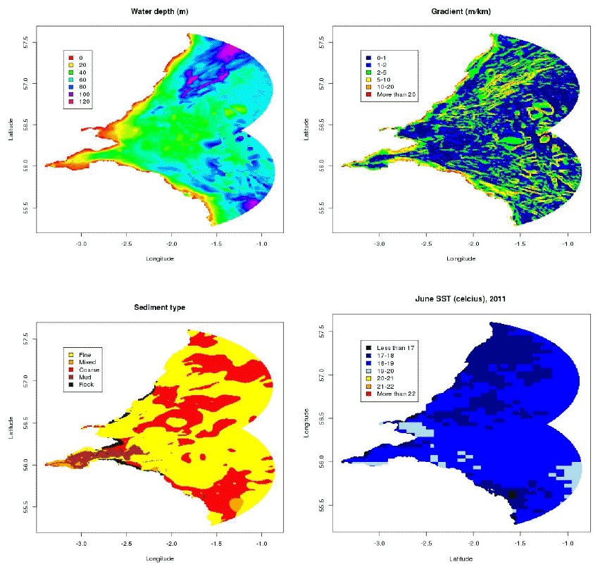
Figure A. 1 shows the spatial distribution of the four variables over the region of interest. Water depth generally increases with distance to coast, but there are extensive areas of shallow water around the coasts of the Firth of Forth and Firth of Tay and areas of deeper water in the NE and SE of the region of interest. Spatial variations in depth gradient are relatively complex, but there are areas of high gradient in both coastal and offshore areas. The majority of the region of interest is covered by two sediment type classifications - coarse and fine/sandy - but the Firth of Forth is predominantly classified as 'Mud'. The remaining two classifications ('rock' and 'mixed') have very limited spatial extent within this region. Spatial variations in SST vary substantially from year to year, with different overall spatial patterns occurring in 2010, 2011 and 2012.

Figure A. 1. Variation in water depth (upper left), seabed gradient (upper right), seabed sediment (lower left) and sea surface temperature in June (lower right) within the study area; example is from 2011.

A.2. Habitat association model

We use a statistical model to describe the relationship between the amount of bird foraging activity and the spatial characteristics of each location within the region of interest. This relationship is assumed to depend on the colony from which birds originate, and the simplest model (our basic model) assumes that the density is determined solely be the distance to the colony:

foraging bird density = a * (Distance to colony) ^b

The effect of distance from colony is expected to strong during the breeding season (the period for which we have data) because seabirds are central place foragers.

This basic model is then modified to account for the effects of environmental variables, by including an additional element in the model to represent spatial variation in the underlying suitability of different locations.

foraging bird density = a * (Distance to colony) ^b * suitability

The basic model is equivalent to assuming that the value of suitability is equal to one for all locations. We assume that suitability does not depend on colony - this reflects that idea that suitability is a fundamental characteristic of the location, rather than a characteristic of the birds that feed at it.

The key assumption within this project is that 'suitability' is (approximately) proportional to prey abundance. The GPS data are used to estimate the unknown parameters within the model, which in turn allows us to produce estimate values of suitability for each site - finally, this allows us to produce indirect maps of prey abundance that are used as inputs to the model of seabird displacement.

We assume that suitability depends upon some or all of the four explanatory variables mentioned above. The most complicated model that we consider is of the form

log(suitability) = ₁ * depth + ₂ * gradient + ₃ * sediment type + ₄ * SST

Sixteen possible models were considered, based on all possible combinations of the four environmental variables:

1. Distance to colony (the basic model)

2. Distance to colony + depth

3. Distance to colony + gradient

4. Distance to colony + depth + gradient

5. Distance to colony + SST

6. Distance to colony + depth + SST

7. Distance to colony + gradient + SST

8. Distance to colony + depth + gradient + SST

9. Distance to colony + sediment type

10. Distance to colony + depth + sediment type

11. Distance to colony + gradient + sediment type#

12. Distance to colony + depth + gradient + sediment type

13. Distance to colony + SST+ sediment type

14. Distance to colony + depth + SST+ sediment type

15. Distance to colony + gradient + SST+ sediment type

16. Distance to colony + depth + gradient + SST + sediment type (the most complicated model)

The model is implemented in R using the 'glm' routine. The basic approach is to fit a logistic regression model (Binomial GLM) in which the data consist of observed foraging locations and control points (points on the regular 0.5 x 0.5 min grid that is used for the GEBCO bathymetry data) and the response variable is binary (1 = Case = actual foraging location; 0 = Control = point on the grid). The control data are repeated so as to cover all site-by-year combinations that are contained within the observed data. The basic model contains two explanatory variables: site-by-year combination (a categorical nuisance variable which accounts for differences in the number of GPS tags deployed for different years and sites), and distance to colony. The remaining models additional contain some or all of the environmental variables: water depth (numeric), depth gradient (numeric), June SST (numeric), sediment type (categorical).

A.3. Assessing model performance

To assess model performance we used a cross-validation approach whereby we applied each model to the entire dataset, and then to subsets of the data, omitting either one of the colonies or one of the years. We then compared the predicted and observed bird densities for each model using a statistical measure of similarity (called KL-divergence). We end up with three measures of performance for each model -

1) performance of the model in predicting foraging density for the entire dataset, given that the model was fitted to the entire dataset;

2) performance of the model in predicting foraging density for a year that was omitted from the modelling;

3) performance of the model in predicting foraging density for a site that was omitted from the modelling.

A.4. Results

A.4.1. Habitat suitability

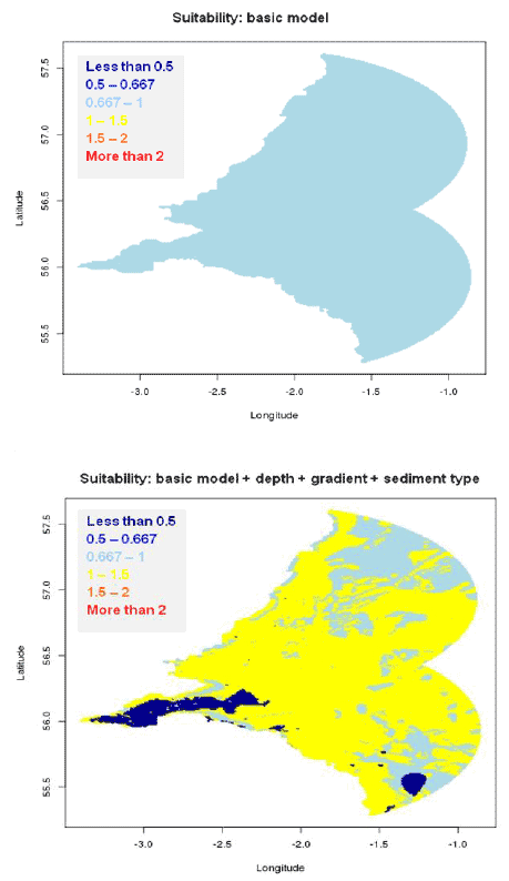
The results of our initial modelling (Figure A. 2) suggest that models which contain sediment type exhibit substantial spatial variation in suitability, whilst those that exclude this variable contain only modest spatial variations. When sediment type is included in the model the areas with lowest suitability are found to be those associated with mud and mixed sediments, whilst the areas with highest suitability are those associated with coarse and fine/sandy sediments. This corresponds, geographical, to the areas of lowest suitability generally occurring in and around the Firth of Forth and the areas of highest suitability generally occurring offshore.

Figure A. 2 Habitat suitability maps of the study area derived from the basic model (upper) and derived from the model including all environmental variables (lower).

A.4.2. Predicted bird density

Suitability is the primary output from our analyses, since it assumed to provide a proxy measure for spatial variations in prey density, but we also use the models to produce predicted maps of bird density. These predictive maps are produced partly in order to summarize the outputs of our analyzes in such a way that they can be checked for biological plausibility.

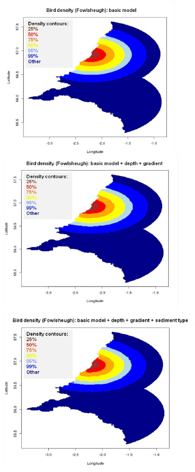
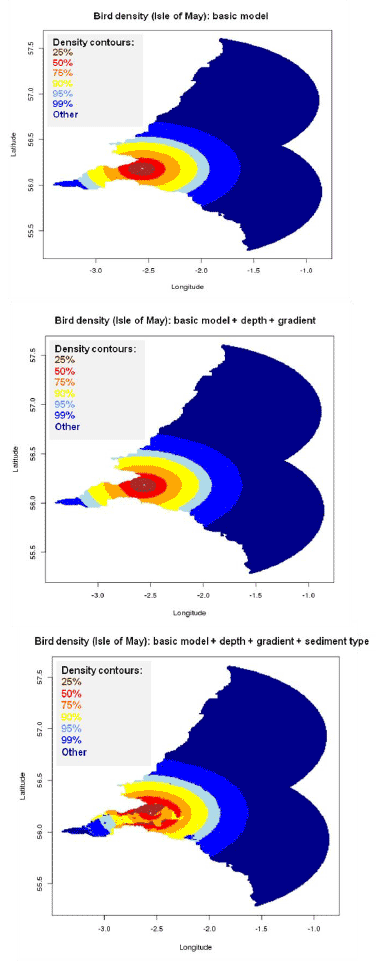
The predicted bird densities for Fowlsheugh (Figure A. 3) are very similar for all of the models that we have considered. The predicted bird densities for the Isle of May (Figure A. 4) are very similar for all models that exclude sediment type, but models that include sediment type show much lower predicted bird densities in areas of mud and mixed sediment than in areas with more common sediment type classifications (sandy/fine and coarse). Both sets of results are derived from the same model, so the large differences in the results that are obtained for the two colonies seem somewhat contradictory. The apparent lack of effect at Fowlsheugh can be explained that mud and mixed sediment type classification are simply not present at all within the areas that are readily accessible from the colony. The results so far have not shown any strong effects of the other environmental variables (depth, gradient or SST).

Figure A. 3. Predicted bird density map around the Fowlsheugh colony derived from the basic model (upper), the model with depth and seabed gradient (middle) and the model with depth, seabed gradient and sediment type (lower).

Figure A. 4. Predicted bird density map around the Isle of colony derived from the basic model (upper), the model with depth and seabed gradient (middle) and the model with depth, seabed gradient and sediment type (lower).

A.5. Interpretation

Sediment type is by the far the most important environmental variable in the models, and the best model contains just this one variable. The model with sediment type remains the best model if we assess performance against years that have been left out, suggesting there is no interannual variation in the importance of this variable (Table A. 2). However, models containing sediment type perform very poorly if performance is assessed against sites that have been left out (Table A. 2). Possible explanations for this are: 1/ the accessibility of sediment types differs widely between colonies, with all types of sediment only present around the Isle of May mainly fine and coarse sediments present in the areas surrounding the other two colonies; 2/ the 'sediment type' effect reflects a geographical effect of coastal features around the different colonies rather than a true effect of seabed sediment.

Table A. 2. Percentage change in model performance relative to the basic model.

Model	All data	Omitting colonies	Omitting years
Dist	0	0	0
Dist + depth	-0.08	-0.82	-0.25
Dist + gradient	-0.08	-0.53	0.16
Dist + depth + gradient	-0.12	-1.54	0.05
Dist + sediment	0.67	-30.26	1.11
Dist + depth + sediment	0.57	-32.08	1.04
Dist + gradient + sediment	0.54	-30.48	0.89
Dist + depth + gradient + sediment	0.44	-31.98	0.90
Dist + SST	-0.05	-0.15	-0.13
Dist + depth + SST	-0.19	-1.19	-0.57
Dist + gradient + SST	-0.06	-0.71	0.12
Dist + depth + gradient + SST	-0.15	-1.98	-0.15
Dist + sediment + SST	0.56	-30.83	0.94
Dist + depth + sediment + SST	0.39	-32.94	0.71
Dist + gradient + sediment + SST	0.49	-31.03	0.80
Dist + depth + gradient + sediment + SST	0.34	-32.80	0.66