Scottish Marine and Freshwater Science Vol 6 No 6: Development of a Model for Predicting Large Scale Spatio-Temporal Variability in Juvenile Fish Abundance from Electrofishing Data

Model Fitting: A Case Study Using 0+ Atlantic Salmon

To demonstrate the modelling approaches described in this report an analysis of salmon fry abundance was undertaken. All potential covariates (see above) were included during model selection for both capture probability and density with the exception of Organisation, which was only included in the capture probability model because it should not affect fish density; and catchment that was only included in the density model because there were not electrofishing observations in all catchments resulting in over fitting. Given the large number of potential interaction terms only main effects were considered.

Data coverage

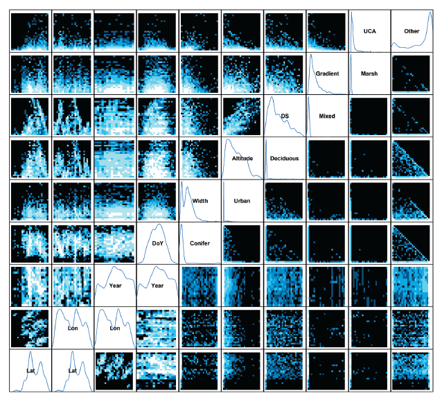
Pairwise density plots of the data coverage in relation to covariates are presented in Figure 8. Latitude and Longitude have been included to identify the spatial coverage of available data, although they were not included as covariates during model fitting. The plots highlight where combinations of covariate values are well represented, for example low slopes and short distance to sea. But also where combinations are absent or rare, for example low elevation, high distance to sea. In addition, some combinations of land use variables are not possible because the landuse combinations need to sum to 100%.

Capture probability

The final capture probability model was selected using a step-wise selection procedure based on minimum BIC, where the initial model had a common capture probability across all site visits. Organisation and Year were included as factors. Year was included as factor to allow for inter-annual variability in hydrological conditions and on the assumption that there would be no reason to assume long-term trends in capture probability. HA was included as a spatial effect. All remaining continuous variables were included as both linear effects and as smoothers with 2 degrees of freedom. The final model was:

logit p ~ Organisation + s(DoY) + Year + regional( HA) + DS + Width + s(Gradient)

The relative importance of explanatory covariates was assessed by dropping terms one at a time from the final model. The importance of terms in the final model was indicated by the magnitude of changes in BIC with more important terms associated with greater changes ( Table 1). Organisation was the most important covariate, followed by DoY, Year, DS, Width and Gradient. The addition of Gradient has a minimal effect on the fit.

Covariate	Degrees of Freedom	Change in BIC
Organisation	23	889.2
s(DoY)	2	438.1
Year	16	207.4
regional( HA)	7	176.2
DS	1	57.3
Width	1	27.7
s(Gradient)	2	0.6

Table 1 The relative importance of explanatory covariates in the capture probability model as indicated by changes in BIC where single terms were removed from the final model. The degrees of freedom shows the reduction in parameters associated with removing the term.

Figure 8 Density plots showing the distribution of available data in relation to combinations of environmental covariates (white: lots of data, blue: few data, black no data). Latitude (Lat) and Longitude (Lon) are included to provide an indication of spatial coverage although these were not included in model fitting.

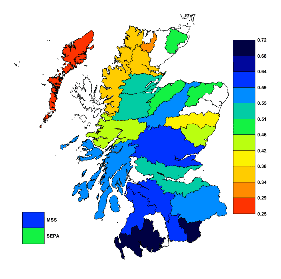
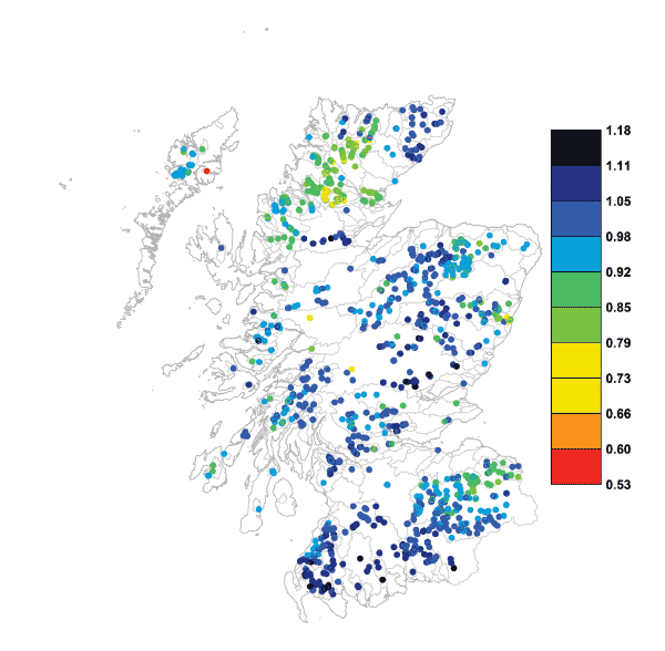
Figure 9 Estimates of capture probability by data provider (Organisation). Estimates are plotted in relation to the geographic area of responsibility ( e.g., Trust Boundaries) of each organisation, although data coverage may be broader. Note that the Galloway Fisheries Trust covers the Galloway region and the Border Esk to the East. White areas indicate either no multi-pass fishing data or no data provider present in that region. In the case of the River Don, permission to use available data came too late to include in this report. MSS and SEPA estimates are indicated to the side of the map given their wide ranging data coverage. Estimates are conditioned on HA Tay, Year 1996 and median values for all remaining covariates. Missing estimates reflect a lack of data availability at the time of model fitting. Map based on digital spatial data licensed from Centre for Ecology and Hydrology, © NERC.

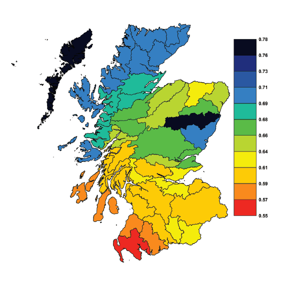
Figure 10 Estimates of spatial variability in capture probability ( HA). Estimates are conditioned on Year 1996, Organisation MSS, and median values for all remaining covariates. Map based on digital spatial data licensed from Centre for Ecology and Hydrology, © NERC.

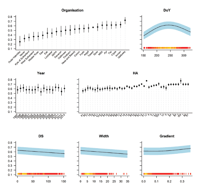
Figure 11 Relationships between capture probability and covariates. Plots are conditioned on HA Tay, Organisation MSS, Year 1996, and median values for remaining covariates. Organisation names have been abbreviated. HA values are ordered from South to North. 95% pointwise confidence intervals are shown as shaded blue areas or vertical bars. A 'rug' indicates the distribution of available data on the x-axis (red: few values, yellow: many values).

Figure 12 Map showing proportional differences in density estimated using a constant mean capture probability (0.53) and modelled capture probabilities. Higher values indicate higher modelled densities relative to constant capture probability. Map based on digital spatial data licensed from Centre for Ecology and Hydrology, © NERC.

Organisation had the greatest effect on capture probability, potentially reflecting differences in equipment and procedures between data providers (Fig. 9 & 11). The next strongest effect related to the time of sampling (DoY). This had a modal effect of similar magnitude which increased from day 150 to ca. 240 and declined thereafter ( Fig. 11). Year had a substantial effect, but showed no temporal trends. HA also had an effect of similar magnitude to year, but also showed an increasing trend in capture probability from south to north (Fig. 10 & 11). The remaining effects were relatively small. Catch probability showed a negative linear response to DS and Width and a positive non-linear response to Gradient.

Figure 12 demonstrates the importance of including catch probability in estimates of fish density. Densities were estimated for each site assuming 1) modelled capture probabilities and 2) a constant capture probability of 0.53 (the mean of the modelled capture probabilities). The plotted differences indicate where modelled capture probabilities result in proportionately greater (>1) or lower (<1) estimates of density. Clear spatial patterns can be observed in the resulting difference plot indicating that a failure to account for variation in capture probability would result in biased estimates of density and potentially misleading spatio-temporal models.

Density

Because the density model was fitted as a GAM it was possible to use ridge regression to drop terms in a form of automatic model selection (Wood, 2006). Models were fitted using Restricted Maximum Likelihood ( REML) assuming a negative binomial distribution to allow for over-dispersion. Any retained terms where the degrees of freedom were estimated to be one or less were replaced by linear terms. The number of degrees of freedom was restricted to a maximum of 3 for all continuous variables. The HA spatial smoother was restricted to a maximum 24 degrees of freedom. The final model was:

log density ~ random(Catchment) + random(Year) +
s(DoY) + s(Width) + s(Altitude) + s( DS) +
Gradient + s( UCA) + Urban + Conifer +
s(Mixed) + s(Other)

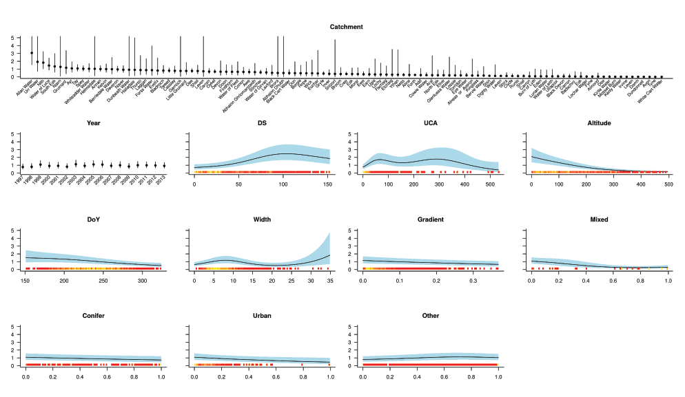
Catchment and Year had substantial spatial and temporal effects on fish density respectively, although there was no evidence of a long-term trend in the data i.e. year was retained as a random effect, but not a temporal smoother (Fig. 13 & 14). The greatest "habitat effects" were associated with DS, UCA and Altitude, which exhibited asymptotic and, complex non-linear and decreasing non-linear responses respectively ( Fig. 13). DoY and Width were the next greatest effects. The effect of river Width was modal around 8m, but was highly uncertain above ca. 25m, where there were very few data, and observations may reflect difficulties in assigning appropriate Widths or biased partial sampling of wider rivers (see section 'Sources of Error in Covariates'). Density estimates exhibited a negative non-linear trend with DoY. The remaining effects (Gradient, % Mixed Woodland, % Conifer Woodland, % Urban and % Other landuses) were substantially smaller and negative with the exception of Other. Percentage Marsh, Deciduous woodland and HA were dropped from the final model.

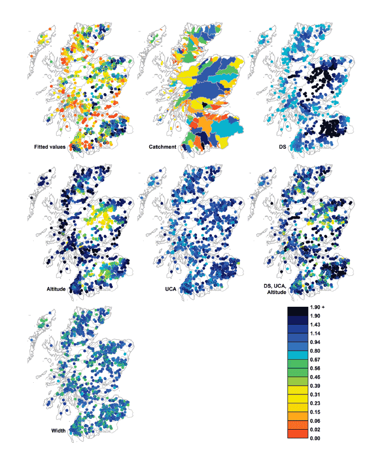
The fish density model predicted spatially heterogeneous fish densities, although the highest densities were usually predicted for large east coast rivers, with lower densities generally in the central belt and west coast (see Figure 14: Fitted Values). To improve understanding of the effects of individual covariates on the spatial distribution of densities, their conditional effects were explored ( Fig. 14).

The effects of catchment were highly heterogeneous with nearby catchments often exhibiting strongly contrasting effects e.g., the Nith and Kirkubrightshire Dee. However, catchment effects were generally negative in the central belt reducing density expectations in these areas.

The effect of DS was to increase densities in inland areas of larger east coast catchments ( Fig. 14: DS). In contrast, low altitude areas were predicted to have higher densities and these were observed near the coast of all rivers ( Fig. 14: Altitude). The effect of UCA was to mirror DS, increasing predicted densities in larger rivers close to the sea, but also favouring overall densities in large dendritic rivers such as the Tweed. Given the spatial correlations between DS, Altitude and UCA, it is useful to see the combined effects of these variables which reduced predicted densities in major upland areas such as the Cairngorms and predicted higher densities in lowland and coastal areas ( Fig. 14: DS, UCA, Altitude). Given the modal effect of width, the spatial distribution of effects was highly heterogeneous ( Fig. 14: Width).

Figure 13 Relationships between fish density and covariates. Plots are conditioned on Catchment Tay, Year 1996, and median value for all remaining covariates. Catchment names are abbreviated. 95% pointwise confidence intervals are shown shaded in blue. For continuous covariates a 'rug' showing the distribution of available data is overlaid on the x-axis (red: few data, yellow: much data, white: no data). High observations for % Urban area represent groups of observations with similar values rather than single observations.

Figure 14 Maps showing the modelled effects of covariates (individual covariates and in-combination) on the spatial distribution of salmon fry densities. Model predictions are conditioned on Catchment Tay, Year 1996, and the median value for remaining covariates. Map based on digital spatial data licensed from Centre for Ecology and Hydrology, © NERC.

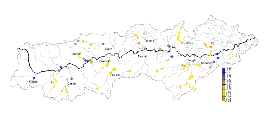
Figure 15 Performance of River Dee monitoring sites relative to the national expectation averaged across years. Coloured points indicate the difference between the predicted salmon fry densities from the national model (accounting for variability in habitat) and smoothed model residuals (fitted using the RC) including the effect of Catchment. Yellow points indicate that sites meet an average national expectation over the monitoring period, orange indicate lower than expected, green and blue higher than expected. Light lines indicate tributaries, the bold line indicates the mainstem river as defined by the SEPA river lines dataset. Map based on digital spatial data licensed from Centre for Ecology and Hydrology, © NERC.

Having accounted for large scale spatial, temporal and habitat covariates, within river variability can remain in the form of network spatial correlation. This variation can be described using the RC smoother. Although it wasn't possible to fit this term to all rivers in Scotland, it was possible to demonstrate the effect for a single river catchment (the Aberdeenshire Dee). This was achieved by fitting RC to the density residuals for the Dee which results in a smoothed residual representation of the average (site-wise) deviations from model predictions ( Fig. 15). Put more simply, the river smoother represents the within catchment deviation from the average national habitat model averaged over time. When combined with the catchment effect, the resulting predictions indicate the differences in density between average model predictions for Scotland and those for the Dee. Figure 15 suggests that salmon fry densities in the Dee are generally as expected (yellow) or better (yellow-green to blue) than would be expected from the mean national model with no marked spatial patterns, although poorly performing sites (orange) were only present in the lower half of the catchment.

Although RC was illustrated here using an average performance metric, it would also be possible to make predictions for the best year nationally (highest densities) and then investigate model residuals for each monitoring year individually. This would assess performance of monitoring sites relative to the best observed conditions and permit assessment of spatial variability in performance over time.