Scottish Marine and Freshwater Science Vol 6 No 14: Developing an avian collision risk model to incorporate variability and uncertainty
The report describes the data required, and the methods used, to estimate collision
risk. It is accompanied by a worked example and R code (available at
http://dx.doi.org/10.7489/1657-1), which enables the collision risk calculations to be
performed in
Part 2: Worked Example
Downloading R
Whereas previous iterations of the Band model have used Microsoft Excel, the collision risk model update presented uses R. To get the most recent version of R, go to the R website http://www.r-project.org and click the ' CRAN' link on the left hand side. Select a mirror site near you from the list provided, click the 'Windows' link on the next page, then the 'base' link on the following page, and then download the R installer from the link 'Download R 3.1.2 for Windows' (note that the version number you see may be different than this example).
The collision risk model (available at http://dx.doi.org/10.7489/1657-1) requires the installation of an R package "msm" to allow sampling from a truncated normal distribution. This should be installed before the model is run.
To install the required package type the following
install.packages("msm")
into the R console and press return.
Once installed, this step should not be required again and the package will be loaded from within the model script.
Imagined scenario
This example is fictitious. The results are not characteristic of collision risks at any particular site.
A wind farm is planned for the North Sea. The imagined area has a width of 10 km and it is intended that the planned wind farm will generate 600 MW. The location of the development area is at 55.8 degrees latitude and has a tidal offset of 2.5 metres. One of the seabirds present at the site and considered sensitive to collision risk is the black-legged kittiwake ( Rissa tridactyla). This worked example estimates a collision risk estimate for kittiwake.
The wind farm is still in the design phase and there is some uncertainty surrounding the turbine design.
The collision risk model
The collision risk model update is provided as R code. The majority of the model is written as functions which are provided in individual files in a folder named 'scripts'. These files do not need to be altered. In terms of code, the ONLY file that needs to be altered in order to run the collision risk model is "BandModel.R". All other files are called from R within this script.
In addition to a folder called 'scripts' and the code BandModel.R, there should also be a folder named 'data' that contains the data files required to run the model. The folder should contain the following:
*BirdData.csv - contains the biometric & flight speed data for species of interest. At present data for 12 species are included (Fulmar, Gannet, Lesser Black-backed Gull, Herring Gull, Great Black-backed Gull, Black-legged Kittiwake, Guillemot, Razorbill, Little Auk, and Puffin)
Species can be added as required, however, it is not necessary to remove data for species which are not being considered. It is important that the species names used are taken from the file BirdData.csv and are used throughout, otherwise the model will not recognise the species. The species names used in the code are as follows:
| Species (scientific name) | Code name used in model |
|---|---|
| Fulmar ( Fulmarus glacialis) | Northern_Fulmar |
| Gannet ( Morus bassanus) | Northern_Gannet |
| Lesser Black-backed Gull ( Larus fuscus) | Lesser_Black_Backed_Gull |
| Herring Gull ( Larus argentatus) | Herring_Gull |
| Great Black-backed Gull ( Larus marinus) | Great_Black_backed_Gull |
| Black-legged Kittiwake ( Rissa tridactyla) | Black_legged_Kittiwake |
| Guillemot ( Uria aalge) | Common_Guillemot |
| Razorbill ( Alca torda) | Razorbill |
| Little Auk ( Alle alle) | Little_Auk |
| Puffin ( Fratercula arctica) | Atlantic_Puffin |
| Arctic skua ( Stercorarius parasiticus) | Arctic_Skua |
| Great skua ( Stercorarius skua) | Great_Skua |
*CountData.csv - count data for the species of interest, should be entered as densities (Birds/km 2). Make sure that biometric data for each species included here is available in BirdData.csv
*FlightHeight.csv - modelled flight height distributions for 21 species of seabird/seaduck etc. taken from Johnston et al. (2014)
*TurbineData.csv - should contain information on the size etc. of the turbines being considered. Each row represents a different turbine model to be considered. The name should be the MW rating of the turbine.
* [insert species name]_ht.csv - should contain bootstrapped flight height distribution data from Johnston et al. (2014) for the species required. A separate file is required for each species.
* windpower_[insert turbine model name].csv - should contain the relationship between wind speed, rotor speed and pitch. A separate file is required for each turbine model/type.
Data requirements
BIRD DATA: these data are entered in to BirdData.csv
Bird length (Body_Length, Body_LengthSD): the bird body length data were taken from the Concise Birds of the Western Palearctic ( OUP, 1994), BTO bird facts and other sources. A mean and standard deviation were estimated from these sources. Mean = 0.39 metres, standard deviation = 0.005.
Wing span (Wingspan, WingspanSD): the wing span data were taken from the Concise Birds of the Western Palearctic ( OUP, 1994), BTO bird facts and other sources. A mean and standard deviation were estimated from these sources. Mean = 1.08 metres, standard deviation = 0.04.
Flight speed data (Flight_Speed, Flight_SpeedSD): the flight speed data used in this worked example were taken from the RSPB FAME project and were collected using GPS tags. The data were used to parameterise a normal distribution. A mean flight speed for each tagged bird was estimated (to remove variation within individual) and then an overall mean of these values was calculated. Mean = 7.26 m.s -1, standard deviation = 1.5.
Nocturnal activity (Nocturnal_Activity, Nocturnal_ActivitySD): the data used in this worked example to estimate the proportion of nocturnal activity were taken from the RSPB FAME project and were collected using GPS tags. All records away from the nest and travelling at speeds considered to be flying were used. The data were used to parameterise a normal distribution. Mean = 0.033, standard deviation = 0.0045.
Proportion at collision risk height (Prop_CRH_Obs, Prop_CRH_ObsSD): these data are required for the basic model (option 1). A mean and standard deviation were calculated using the data within Black_legged_Kittiwake_ht.csv. For each bootstrapped distribution curve, the proportion of birds between the average minimum and average maximum rotor tip height was summed. From these values, a mean and standard deviation was calculated. Mean = 0.06, standard deviation = 0.009.
Avoidance (AvoidanceBasic, AvoidanceBasicSD, AvoidanceExtended, AvoidanceExtendedSD): This is the probability that a bird on a collision course with a turbine will take evading action to avoid collision. The data were taken from Cook et al. (2014) and for kittiwake, we used the 'all gulls' avoidance rate. The avoidance rate differs between the basic and extended models and a mean and standard deviation are required for both. Mean (basic) = 0.9893 and standard deviation (basic) = 0.0007; mean (extended) = 0.9672 and standard deviation (extended) = 0.0018.
COUNT DATA: these data are entered in to CountData.csv and are the number of birds in flight in the daytime presented as birds/km 2. A mean and standard deviation are required. For this worked example, data were taken from the Creyke Beck A Environmental Statement.
| Month | Mean | SD |
|---|---|---|
| Jan | 0.97 | 0.67 |
| Feb | 1.04 | 0.75 |
| Mar | 1.15 | 0.78 |
| Apr | 0.48 | 0.36 |
| May | 0.56 | 0.58 |
| Jun | 0.63 | 0.45 |
| Jul | 0.68 | 0.47 |
| Aug | 0.64 | 0.47 |
| Sep | 0.53 | 0.39 |
| Oct | 1.20 | 0.78 |
| Nov | 1.02 | 0.61 |
| Dec | 0.99 | 0.7 |
FLIGHT HEIGHT DISTRIBUTION DATA: these data are contained within FlightHeight.csv and the individual species files such as Black_legged_Kittiwake_ht.csv and are required for options 2 and 3. The data within FlightHeight.csv are provided by the British Trust for Ornithology (Johnston et al, 2014) and are generic flight height distributions. The file provides data on the proportion of birds within 1m height bands for 21 species. For example,
| Height (m) | Black_legged_Kittiwake |
|---|---|
| 1 | 0.089904 |
| 2 | 0.081107 |
| 3 | 0.072538 |
| 4 | 0.067068 |
| 5 | 0.061008 |
| 6 | 0.055579 |
| 7 | 0.050707 |
| … | … |
Confidence intervals were calculated around these best fit/generic flight height distributions using a bootstrapping approach, randomly sampling from the original dataset each time. These bootstraps are provided for each species in separate files, for example Black_legged_Kittiwake_ht.csv and are used to include uncertainty surrounding the flight height distribution.
TURBINE DATA: these data are entered into TurbineData.csv and are also contained within the turbine-specific files such as windpower_6. Names in parentheses are the names in the data files and scripts.
Rotor radius (RotorRadius, RotorRadiusSD): this is measured from the axis of rotation to blade tip and was taken from expert opinion. Mean = 80 and Standard deviation = 5
Hub height (HubHeightAdd, HubHeightAddSD): This is the measure that in addition to rotor radius sums to give the distance from HAT to the axis of rotation and was taken from expert opinion. Mean = 26.5 and Standard deviation = 2.
Maximum blade chord width (BladeWidth, BladeWidthSD): This is the maximum width of the rotor blade and was taken from expert opinion. Mean = 5.5 and Standard deviation = 0.3.
Turbine operation time (example for January is JanOp, JanOpMean, JanOpSD): This included both information on wind availability (JanOp) which is considered a constant and maintenance down time (JanOpMean, JanOpSD) which included uncertainty. Data were taken from the Inch Cape Environmental Statement.
| Month | Wind availability | Mean maintenance | SD maintenance |
|---|---|---|---|
| Jan | 96.28 | 6.3 | 2 |
| Feb | 96.53 | 6.3 | 2 |
| Mar | 95.83 | 6.3 | 2 |
| Apr | 92.78 | 6.3 | 2 |
| May | 90.86 | 6.3 | 2 |
| Jun | 92.22 | 6.3 | 2 |
| Jul | 89.11 | 6.3 | 2 |
| Aug | 89.92 | 6.3 | 2 |
| Sep | 93.71 | 6.3 | 2 |
| Oct | 96.14 | 6.3 | 2 |
| Nov | 97.14 | 6.3 | 2 |
| Dec | 96.41 | 6.3 | 2 |
Rotation speed (RotationSpeed, RotationSpeedSD): It is possible to specify a mean rotor speed and standard deviation, however the default model uses the relationship between wind speed and rotor speed provided to calculate the specific rotor speeds, therefore RotationSpeed and RotationSpeedSD in TurbineData.csv should be left blank. The relationship should be provided in a csv file named windpower_[insert model name here] for example windpower_6.csv
The table below shows an example relationship between wind speed, rotor speed and pitch. It was constructed using expert opinion as an example table and used within this worked example. It does not relate to a specific turbine specification currently available.
| Wind speed (m/s) | Rotor Speed | Pitch |
|---|---|---|
| 0 | 0 | 90 |
| 1 | 0 | 90 |
| 2 | 0 | 90 |
| 3 | 6 | 0 |
| 4 | 6 | 0 |
| 5 | 6 | 2 |
| 6 | 8 | 4 |
| … | … | … |
Blade pitch (Pitch, PitchSD): As for rotor speed, it is possible to specify a mean pitch and standard deviation, however the default model uses the relationship between wind speed and pitch provided to calculate the specific rotor pitch, therefore Pitch and PitchSD in TurbineData.csv should be left blank. The relationship should be provided in a csv file named windpower_[insert model name here] for example windpower_6.csv (as above).
Model set up
Before the model can be run it requires information to be entered into the file "BandModel.txt".
1. Set working directory
First, set the working directory. This is the location where the folders 'scripts' and 'data' have been saved as well as 'BandModel.R'. For example,
setwd("F:\\BAND CRM For R")
This step directs R to all the files and data that are required to run the model therefore all the files required much be within this directory.
2. Set results folder
The model will save output to a folder. Set the name of the results folder, for example, the name of the development. For example,
results_folder <- "windfarm1"
If no name is specified the model will default to the date. WARNING: If the model is run several times on the same day and no folder name is specified, it will over-write files in the folder.
3. Set model components
Next set the model components. These include:
The number of iterations the model simulation will execute, for example 1000
iter<- 1000
The species to include, for example kittiwake
CRSpecies = "Black_legged_Kittiwake"
If more species were to be included this would look like
CRSpecies = c("Black_legged_Kittiwake", "Northern_Gannet", "Arctic_Skua")
The target power (in MW) to be generated within wind farm, for example 600 MW. This is used in conjunction with the turbine name i.e. 6 if a 6 MW turbine, to calculate the number of turbines in the array.
TPower = 600
Large array correction (Yes/No), for example
LargeArrayCorrection = "yes"
The wind farm width (km), for example 10km
WFWidth = 10
The proportion of bird flights up/downwind, for example 50%
Prop_Upwind = 0.5
The latitude of the wind farm in decimal degrees, for example 55.8 degrees. This is used to calculate day length at the site location throughout the year.
Latitude = 55.8
The tidal offset in metres (to correct for flight heights being calculated in relation to mean sea-level and turbine dimensions being calculated in relation to Highest Astronomical Tide), for example 2.5 metres
TideOff = 2.5
4. Parameterise wind speed sampling distribution
The model uses wind speed data to calculate rotor speed and pitch. Wind speed data are therefore required. At the time of production it was unclear what format wind speed data would be available to wind farm developers. To avoid inconsistencies, the model samples wind speed from a truncated normal distribution parameterised by the user. The mean wind speed (m.s -1) and standard deviation are required to be set, for example
windSpeedMean<- 7.74
windSpeedSD<- 3.2
It is expected that these will be obtained from met mast data or other sources of wind speed data such as NASA's Modern-Era Retrospective Analysis for Research and Applications ( MERRA).
5. Running the model…
Once you have set the working directory and entered all of the necessary information, all that is needed to run the model is to copy and paste all of BandModel.R into the R console, or alternatively type
source("*****EnterMyDirectoryHere****\\BandModel.R")
in the R console, and press return.
The code is designed to loop through multiple species and multiple turbine designs in a single step. The number of results obtained will depend on the number of different turbine designs entered in TurbineData.csv and the number of different species for which data are entered and listed.
A progress bar will provide an indication of progress and at the end of the model, the time elapsed since the model was started will be displayed.
Model Output
The model outputs information on the expected numbers of collisions. The information is provided both as tables and figures, and according to the species and turbine designs entered into the model. Results are provided for the basic (options 1 and 2) and extended (option 3) versions of the model.
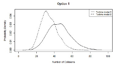
- Option 1 - using the basic model, i.e. assuming that a uniform distribution of flight heights between the lowest and the highest levels of the rotors and using the proportion of birds at risk height as derived from site survey.
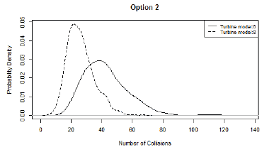
- Option 2 - again using the basic model, but using the proportion of birds at risk height as derived from the generic flight height distribution provided.
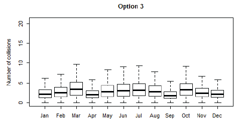
- Option 3 - using the extended model and using the generic flight height distribution.
Tables
The file names of the tables indicate the type of information contained.
1. CollisionEstimates.csv: Overall summary table of collisions by species, turbine and model option. Results are presented as mean, standard deviation ( SD) and coefficient of variation ( CV), and median and inter quartile range ( IQR).
| Species | Turbine | Option | Mean | SD | CV | Median | IQR |
|---|---|---|---|---|---|---|---|
| Black_legged_Kittiwake | 6 | 1 | 45.6455 | 12.5448 | 27.4831 | 45.1206 | 16.5493 |
| Black_legged_Kittiwake | 6 | 2 | 42.4292 | 14.5621 | 34.3210 | 40.3032 | 18.671 |
| Black_legged_Kittiwake | 6 | 3 | 35.4131 | 13.1271 | 37.0685 | 33.0278 | 16.466 |
2. 6_Black_legged_Kittiwake_monthlySummaryOpt1.csv : monthly summaries of collisions. Separate tables are produced according to species, turbine and model option. Results are presented as mean, standard deviation ( SD) and coefficient of variation ( CV), and median and inter quartile range ( IQR).
| Month | Mean | SD | CV | Median | IQR |
|---|---|---|---|---|---|
| Jan | 3.080382 | 1.753642 | 56.92937 | 2.970413 | 2.441757 |
| Feb | 3.590156 | 2.012736 | 56.06263 | 3.439408 | 3.043374 |
| Mar | 4.884338 | 2.76244 | 56.55711 | 4.716011 | 4.134139 |
| Apr | 2.890070 | 1.763726 | 61.02710 | 2.648057 | 2.297968 |
| May | 4.255352 | 2.845274 | 66.86343 | 3.771635 | 3.664073 |
| Jun | 4.458946 | 2.63927 | 59.19044 | 4.172458 | 3.708436 |
| Jul | 4.529034 | 2.769847 | 61.15756 | 4.132559 | 3.751684 |
| Aug | 4.034511 | 2.423247 | 60.06296 | 3.738152 | 3.239942 |
| Sep | 2.720596 | 1.625044 | 59.73115 | 2.546583 | 2.131306 |
| Oct | 4.650331 | 2.451314 | 52.71267 | 4.471203 | 3.288374 |
| Nov | 3.484131 | 1.787375 | 51.30045 | 3.386141 | 2.557487 |
| Dec | 3.067742 | 1.625422 | 52.98432 | 2.964345 | 2.258359 |
3. 6_Black_legged_Kittiwake_sampledBirdParameters.csv: Summary of sampled bird parameters by species, turbine & model option presented as mean & standard deviation ( SD), and median & interquartile range ( IQR).
| Parameter | Mean | SD | Median | IQR |
|---|---|---|---|---|
| AvoidanceBasic | 0.989328 | 0.000696 | 0.989341 | 0.000986 |
| AvoidanceExtended | 0.967215 | 0.00176 | 0.967172 | 0.00244 |
| WingSpan | 1.079481 | 0.040021 | 1.078701 | 0.054751 |
| BodyLength | 0.3898 | 0.005124 | 0.389929 | 0.007007 |
| PCH | 0.06006 | 0.009073 | 0.06025 | 0.012644 |
| FlightSpeed | 7.242055 | 1.472594 | 7.200565 | 1.91039 |
| NocturnalActivity | 0.033239 | 0.004627 | 0.033195 | 0.005833 |
4. 6_Black_legged_Kittiwake_sampledTurbineParameters.csv: Summary of sampled turbine parameters by species, turbine and model option presented as mean and standard deviation ( SD), and median and inter quartile range ( IQR).
| Parameter | Mean | SD | Median | IQR |
|---|---|---|---|---|
| RotorSpeed | 7.8795 | 1.187502 | 6.8 | 2.3 |
| RotorRadius | 80.02557 | 4.641109 | 79.93026 | 6.275585 |
| HubHeight | 106.5836 | 4.981272 | 106.4803 | 6.57322 |
| BladeWidth | 5.492034 | 0.293631 | 5.499434 | 0.414762 |
| Pitch | 1.091 | 2.912594 | 0 | 0 |
| JanOp | 90.04184 | 1.992513 | 90.08147 | 2.699385 |
| FebOp | 90.32209 | 2.00625 | 90.27184 | 2.864814 |
| MarOp | 89.53487 | 1.983321 | 89.52079 | 2.567127 |
| AprOp | 86.5725 | 2.050986 | 86.58052 | 2.786068 |
| MayOp | 84.5539 | 1.99842 | 84.5696 | 2.744052 |
| JunOp | 86.04224 | 2.070166 | 86.06471 | 2.915727 |
| JulOp | 82.7399 | 2.025924 | 82.68036 | 2.643739 |
| AugOp | 83.69396 | 2.0276 | 83.71622 | 2.59691 |
| SepOp | 87.46471 | 2.045078 | 87.38634 | 2.880023 |
| OctOp | 89.81123 | 1.95635 | 89.78423 | 2.731423 |
| NovOp | 90.89083 | 1.979187 | 90.93791 | 2.677976 |
| DecOp | 90.04899 | 2.107647 | 90.1124 | 2.786412 |
Figures
1. 6_Black_legged_Kittiwake .jpg: 3-panel boxplots of monthly collisions for model options 1, 2 and 3 by species, and turbine type (included in the file name).
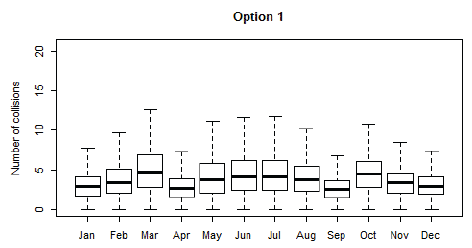
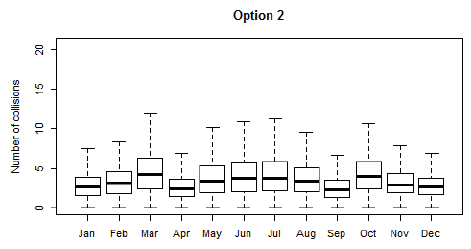
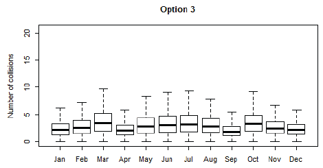
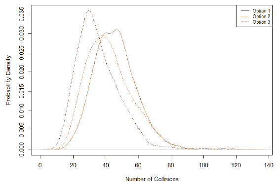
2. 6_Black_legged_Kittiwake_density.jpg: Density plots of numbers of collisions by species, and turbine type (specified in file name). A density curve is plotted for each of the 3 model options.
3. Black_legged_Kittiwake.jpg: If 2 or more turbine models are included, then a 3-panel figure will be produced for each species, with the panels representing model options 1, 2 and 3 and each panel containing probability density plots for the different turbines.
In addition to the collision estimates, the model also saves a copy of the input files which were entered into the model, as well as a summary of the randomly sampled input parameter values. This would therefore allow for the model to be re-run and results verified (if required). It also outputs a text file (run.time.txt) stating the time elapsed between the start and the end of the model, the number of iterations, the species for which the model was run and also the different turbines i.e. 6 MW, 8 MW, etc. if more than one turbine type was specified.
Time difference of 1.936949 hours
"The model ran 1000 iterations"
"The following species were modelled:"
"Black_legged_Kittiwake"
"The following turbines were modelled:"
6 8
A note on comparisons of results: Whilst differences in the density curves (specifically the spread) can be compared within each model option, they should not be compared between different model options. This is because of differences in the way in which variation and uncertainty are introduced into each model option. For example, in the basic model (options 1 & 2) uncertainty in the proportion of birds at risk height is only introduced when estimating the flux rate. However, in the extended model (option 3), the uncertainty in the flight height distribution is introduced when calculating the collision integral (the extended model equivalent of the probability of collision).