Report on razor clam surveys on Tarbert Bank

Materials and methods

Calibration of the video cameras

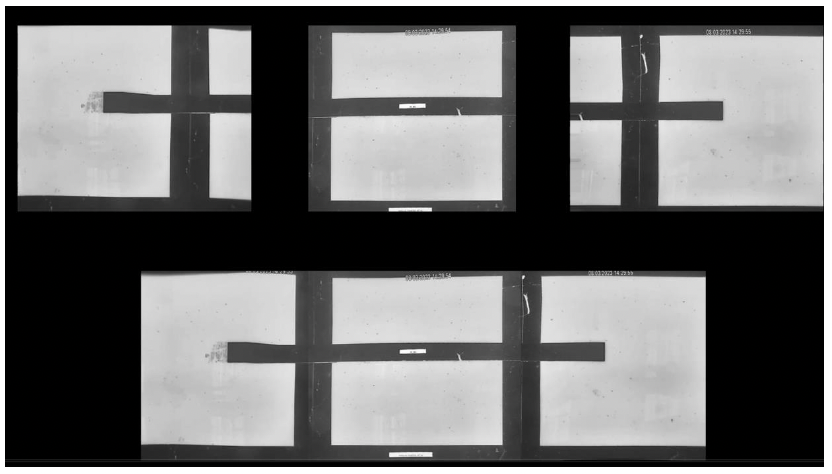
Surveys were conducted using the video equipment described in Fox (2017). Briefly, the equipment consists of three downward pointing cameras mounted on a sled which is towed behind a commercial electrofishing rig. For the Tarbert Bank work the original Sony video cameras were replaced with MacArtney Luxus cameras. Although the Sony cameras were cheap and had provided good service (Fox 2017, Fox 2018, Fox et al. 2019, Fox 2021), they had also not proven to be particularly robust with seawater ingress leading to regular failures. Furthermore, the Sony cameras were no longer available on the market, so an alternative had to be found. The Luxus cameras use the same imaging chip, are better sealed (rated down to 200 m depth), are still relatively inexpensive and could be mounted on the video rig with minor modifications to the mounting brackets. Because new cameras were used in the video rig, it was necessary to recalibrate them using the Scottish Association for Marine Science (SAMS) seawater testing tank prior to the survey. Processing of the video prior to estimating clam sizes involves correcting the video images for camera lens distortion and combining the three separate video feeds to give a composite picture of the video swath. The conversion factor from video pixels to millimetres for the new cameras was estimated to be 1 px = 1.2 mm.

As a further check on the accuracy of reconstructing object sizes from the video, two 150 mm long, plastic blocks were recorded at various locations within the field of view in the test tank. Forty measurements of the blocks at different locations in the field of view were reconstructed from the post-processed video. Compared to the known calibration block length, the reconstructed lengths showed a small positive bias of 3 mm. This probably arises because of the thickness of the blocks which raises them about 1 cm above the test tank floor, and thus above the square calibration targets which are flat and laid underneath the camera rig runners. After applying a 3 mm bias correction, all reconstructed calibration block measurements were within 9 mm of the true block lengths (the mean of the reconstructed measurements = 148 mm, std dev = 4.2 mm, n = 40). The distribution of reconstructed lengths did not differ significantly from a normal distribution (Kolmogorov-Smirnov D = 0.117, p = 0.601) giving a relationship between the 95% confidence interval around a mean against number of objects measured as shown in Figure 2.

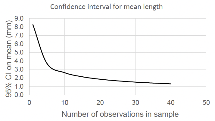
The impact of varying object distance was tested and reported in Fox (2017) for the original Sony cameras. It was concluded that major errors in reconstructed lengths of individual razor clams were unlikely, unless there were large undulations (>5 cm) in the seabed leading to substantial variations in the distance between a camera and the target. Although this source of error was not re-investigated with the MacArtney cameras, the result is expected to be similar following lens distortion correction. The height of sand ripples in the field will generally be smaller than 5 cm, so this is not expected to be a source of significant error in reconstructed object lengths. Individual reconstructed razor clam lengths from field collected video are therefore expected to have an accuracy of ± 9 mm of their true length with the accuracy of mean estimates improving to ± 2 mm (95% confidence interval) when more than 20 observations are included the calculation.

Tarbert Bank field survey

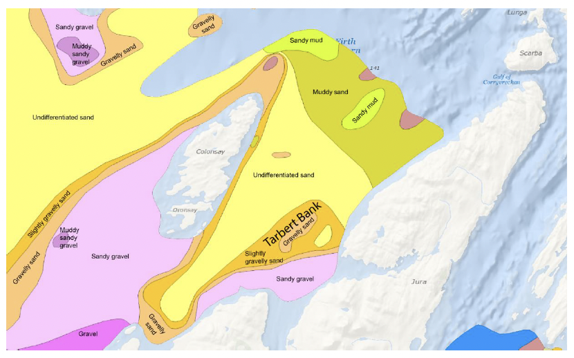
Tarbert Bank lies between the islands of Jura and Colonsay on the Scottish west coast (Figure 3). The permitted area where electrofishing may take place covers waters right around Colonsay, but Tarbert Bank has been a focus of electrofishing effort within this area in recent years.

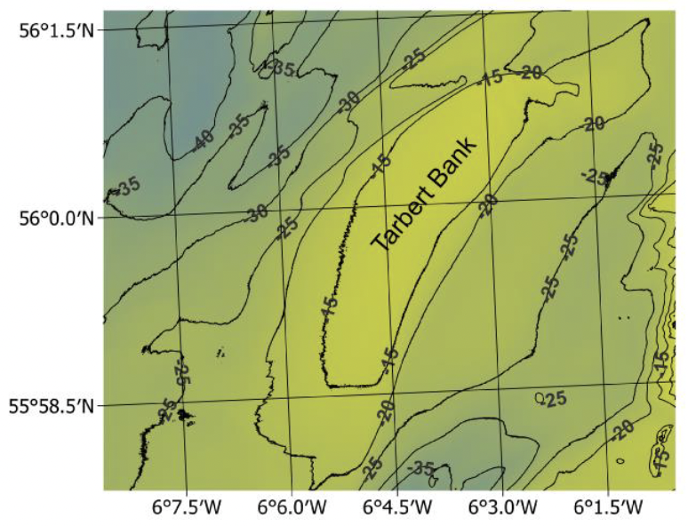
Nearly all the recorded commercial electrofishing has occurred in depths shallower than the 20 m depth contour, and as previously mentioned is restricted to north of latitude 56°N (Figure 4). The bank itself curves slightly towards the south and comprises shallow sandy sediments above 15 m charted depth, dropping away to deeper areas to the northwest and southeast. The area shallower than 15 m is around 5.6 km in north-south direction, and 1.2 km at its widest point. The bank is slightly narrower comparing the northern to the southern sections.

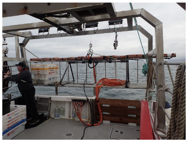
The survey was conducted from the fishing vessel ‘Skye’ (CN450; Scottish Fishing, Campbeltown) skippered by Mr. Craig Barrett. The vessel is new and was built with several features to facilitate electrofishing. These include the general deck layout with the electrode cable connectors conveniently located at the stern, an aft lifting derrick and a stern platform with clips for securing the electrofishing bar when in transit (Figure 5).

The fishing operation involves dropping an anchor and then reversing the vessel whilst paying out a cable until the vessel is between 150 and 200 m from the anchor. ‘Skye’ fishes with a clump weight and therefore relies on a combination of tide and wind to set the direction of the tow. Once the vessel has settled the clump was lowered, the electrofishing gear set on the seabed and the vessel then slowly warped towards the anchor. This means it was not possible to follow a pre-designed survey plan because the exact positions which can be worked are continually varying depending on the changing state of the tide and wind. We therefore placed tows aiming to give a comprehensive coverage of the area. Recovering and moving the anchor is the most time-consuming part of the operation and will reduce the number of tows which can be completed in a day considerably. To reduce the amount of relocation time we collected two or three video tows along each anchor line with tows being spaced at least 50 m apart.

The electrofishing rig consists of a 5 m wide plastic spreader bar fitted with three pairs of brass electrodes, each 2.6 m in length with 1 m separation between positive and negative electrodes. The video rig was towed 3 m behind the spreader bar of the normal commercial electrofishing rig used on ‘Skye’. Power was supplied using an inverter box as 24 V AC at around 50-80 amps per electrode pair in line with the electrofishing equipment regulations stipulated by the Scottish Government for use in the trial fishery. All experimental fishing took place under a specific survey derogation issued by Marine Scotland Access to Sea Fisheries. Once correct deployment of the gear was confirmed (Figure 6), the power to the electrofishing rig was turned on and the survey tows commenced. Maximum fishing depth was around 22 m due to the length of electrode cables available with deeper locations being surveyed at low water. The fishery rarely works areas deeper than 20 m due to the bottom-time limits on air-based SCUBA diving.

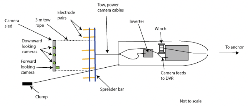
Video from the three downward facing cameras was monitored continuously during the tow and recorded using a digital video recorder (Hawk D1/960H AHD RF3089, RF Concepts, Belfast UK). Water column parameters (temperature and salinity) were recorded daily from the surface to the seabed using a CastAway CTD (SonTek, San Diego, California).

Post fieldwork analysis of recorded videos

Recorded videos were downloaded as .avi files and processed using the Matlab scripts described in Fox (2017), but with the lens distortion calibrations updated for the MacArtney Luxus cameras based on the test-tank calibrations undertaken just before the surveys. The lengths of razor clams on the processed video were recorded manually using the interactive Matlab program which is also detailed in Fox (2017). Additional notes were made of any other organisms seen, such as crabs and fish. All videos were reviewed by the same analyst (Mr Lars Brunner).

To convert the counts to area-based densities, estimates of tow length are required. These were calculated from the start and end positions of each tow recorded from the vessel’s GPS chart plotter. The distance between these two points was calculated using the Haversine formula.

The camera alignments and video processing were set up so that the total imaged swath was 1.5 m wide and thus the swept areas (m²) were estimated as tow lengths multiplied by 1.5 (except for tows on day one of the survey where one of the camera connections failed and the swath width was consequently 1 m in width). Razor clams on the videos were assigned to one of five categories:

1 - whole E. siliqua lying flat on the seabed;

2 - E. siliqua lying flat on the seabed but overlapping the edge of the video frame so that only part of the shell was visible;

3 - Ensis tops where the clam had not fully emerged from the sediment and species could not be indentified;

4 - whole E. magnus lying flat on the seabed;

5 - E. magnus lying flat on the seabed but overlapping the edge of the video frame so that only part of the shell was visible.

For Categories 2 and 5 it was assumed that each count would represent half an individual contribution to the overall density (since on average half an individual count would lie in the adjacent area outside the field of view). The length data from Categories 2 and 5 were not used further. For Category 3, each record was counted as one individual but the total count of category 3 objects on a tow apportioned as to E. siliqua or E. magnus in the ratio of Categories 1:4 in the tow (because it is not possible to reliably discriminate between the species when only the top is visible). The length data for Category 3 were not used further.

Estimation of Ensis densities on Tarbert Bank

To obtain the total count of E. siliqua (all sizes) on tow _i:

E. siliqua _i = count cat 1_i + …

count cat 2_i / 2 + …

count cat 3_i * count cat 1_i / (count cat 1_i + count cat 4i)

Equation [1]

where count Cat 1_i is total number of whole E. siliqua in tow _i; count Cat 2_i is the total number of E. siliqua partially within the video frame in tow _i; count Cat 3 is the total number of partially emerged Ensis in tow _i; and count Cat 4 is the total number of whole E. magnus in tow _i.

When considering the counts and densities of Ensis above a certain length, the count of Category 2 and 3 objects on a tow is meaningless (because the total length of Ensis which are partially within the video frame or partially emerged is not known). The total count above a size limit was thus estimated based on the assumption that the proportional distribution between the size fractions among the different object categories would be the same. Therefore, the total count of E. siliqua above size _z on tow _i is given by:

E. siliqua _{> z, i} = count cat 1 _{> z, i} + …

((count cat 2_i / 2) * (count cat 1 _{> z, i} / count cat 1 _i)) + …

((count cat 3_i * count cat 1_i /( count cat 1_i + count cat 4_i)) * …

(count cat 1 _{> z, i} / count cat 1 _i))

Equation [2]

Density estimates for E. siliqua (nos m^-2) were then calculated by dividing the total counts from tow _i by the estimated swept area of tow _i (m²). Density estimates were mapped using QGIS (version 3.28.4) and other statistical calculations performed using R (version 4.2.2).

Similarly, the total count of E. magnus on each tow was estimated from Equation 3 but because this species is not normally harvested, length stratified counts and density estimates were not produced for this species.

E. magnus _i = count cat 4_i + …

count cat 5_i / 2 + …

count cat 3_i * count cat 4_i / (count cat 1_i + count cat 4i)

Equation [3]

where count Cat 4_i is total number of whole E. magnus in tow _i; count Cat 5_i is the total number of E. magnus partially within the video frame in tow _i.