Production of Seabird and Marine Mammal Distribution Models for the East of Scotland
This report describes temporal and spatial patterns of density for seabird and marine mammal species in the eastern waters of Scotland from digital aerial surveys. This is important in order for the Government to make evidence-based decisions regarding the status of these species and management.
6. Results
Distribution models were produced for ten out of eleven seabird species and three out of four marine mammals. The list of covariates used in the initial models for each species in given in Table 7 and the selected covariates are listen in Table 8 for seabirds and Table 9 for marine mammals.
For seabirds for which it was possible to fit a separate model for breeding and non-breeding season, the model for non-breeding season retained more environmental variables than for breeding season. There was no single environmental covariate which would characterise distribution and density of all seabirds or all marine mammals.
Below we present the results each species: distribution patterns with point estimates and associated uncertainties (confidence intervals and coefficient of variation, CV)
6.1 Adjustments for non-recognition
Table 5 gives the adjustments made for each species due to non-recognition or species grouping. For species such as guillemot, 94% of observed numbers were assigned to species group, rather than species. For a small review of species grouping see Appendix 1.
| Species |
Adjustments |
Non-recognised animals allocated |
Proportion of total* numbers recorded |
| Northern fulmar |
No adjustments made |
0 |
0% |
| Northern gannet |
No adjustment made |
0 |
0% |
| Great skua |
No adjustment made |
0 |
0% |
| Common gull |
Adjusted based on MERP database |
41 |
30% |
| Lesser black-backed gull |
Adjusted based on MERP database |
57 |
63% |
| Herring gull |
Adjusted based on MERP database |
1347 |
42% |
| Great black-backed gull |
Adjusted based on MERP database |
603 |
28% |
| Black-legged kittiwake |
No adjustment made |
0 |
0% |
| Common guillemot |
Adjusted based on MERP database |
1583 |
94% |
| Razorbill |
Adjusted based on MERP database |
30 |
0.04% |
| Atlantic puffin |
Adjusted based on MERP database |
104 |
19% |
| Minke whale |
Adjusted based on MERP database |
6 |
16% |
| Common dolphin |
Adjusted based on MERP database |
0 |
0% |
| White-beaked dolphin |
Adjusted based on MERP database |
306 |
58% |
| Harbour porpoise |
Adjusted based on MERP database |
545 |
56% |
*Knowns and estimated unknowns
6.2 Realised effort
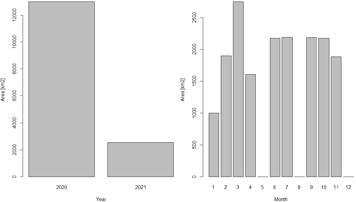
The total effort (as areas) per year and per month is given in Figure 3. The total area surveyed was 16,882.47 km2. The distribution of effort by survey is shown in Table 6 and Figure 6. The was no surveys taking place in May, August and December and February and March were surveyed both in 2020 and 2021.
| Survey |
Time period |
Covered area, as (km2) |
| 1 |
February/March 2020 |
2181 |
| 2 |
April 2020 |
1608 |
| 3 |
June 2020 |
2180 |
| 4 |
July 2020 |
2192 |
| 5 |
September 2020 |
2185 |
| 6 |
October 2020 |
2176 |
| 7 |
November 2020 |
1884 |
| 8 |
February/March 2021 |
2534 |
| Total |
16940 |
Table 7. Initial models including list of environmental covariates for each species. All covariates were fitted as continuous variables (indicated by s()).
Most Birds
breeding season
Initial Model (on scale of link function)
s(Easting, Northing) + s(MeanSSTbymonth) + s(MeanRangeSSTbyMonth) + s(MeanSalinitybyMonth) + s(MeanRangeofSalinitybyMonth) + s(Current) + s(Depth) + s(Seabed Roughness) + s(Simpson Hudson Stratification Index )+s(Colony Index) + offset(log(Km2)),
Non- breeding season
Initial Model (on scale of link function)
s(Easting, Northing) + s(MeanSSTbymonth) + s(MeanRangeSSTbyMonth) + s(MeanSalinitybyMonth) + s(MeanRangeofSalinitybyMonth) + s(Current) + s(Depth) + s(Seabed Roughness) + s(Simpson Hudson Stratification Index ) + offset(log(Km2)),
Birds (reduced dataset (n = 5093)
Initial Model (on scale of link function)
s(Easting, Northing by Season) + s(MeanSSTbymonth by Season) + s(MeanRangeSSTbyMonth by Season) + s(MeanSalinitybyMonth by Season) + s(MeanRangeofSalinitybyMonth by Season) + s(Current by Season) + s(Depth by Season) + s(Seabed Roughness by Season) + s(Simpson Hudson Stratification Index by Season )+s(Colony Index by Season) + offset(log(Km2)),
Minke whale
Initial Model (on scale of link function)
s(Easting, Northing) + s(Dayofyear) + offset(log(Km2))*
Common dolphin
Initial Model (on scale of link function)
s(Easting, Northing) + offset(log(Km2))
White-beaked dolphin
Initial Model (on scale of link function)
s(Easting, Northing) + s(MeanSSTbymonth) + s(MeanRangeSSTbyMonth) + s(MeanSalinitybyMonth) + s(MeanRangeofSalinitybyMonth) + s(Current) + s(Depth) + s(Seabed Roughness) + s(Simpson Hudson Stratification Index ) + offset(log(Km2)),
Harbour porpoise
Initial Model (on scale of link function)
s(Easting, Northing) + s(MeanSSTbymonth) + s(MeanRangeSSTbyMonth) + s(MeanSalinitybyMonth) + s(MeanRangeofSalinitybyMonth) + s(Current) + s(Depth) + s(Seabed Roughness) + s(Simpson Hudson Stratification Index ) + offset(log(Km2))
*s(Depth) was subsequently tried.
Table 8. Selected models for seabirds.
Northern fulmar
Season
Breeding
Final Model (on log scale, offset not shown)
s(Easting, Northing) + MeanMonthlySST + MonthlySalinityRange
No of segments
29291
Correlation structure*
AR1
Assumed error
Negative binomial
Non-breeding
Final Model (on log scale, offset not shown)
s(Easting, Northing) + MeanMonthlySST + SSTMonthlyRange + MeanMonthlySalinity
No of segments
67799
Correlation structure*
AR1
Assumed error
Negative binomial
Northern gannet
Season
All year
Final Model (on log scale, offset not shown)
s(Easting) + s(MeanMonthlySST)
No of segments
5093
Correlation structure*
ARMA(1,1)
Assumed error
Negative binomial
Great skua
Season
All year
Final Model (on log scale, offset not shown)
s(Easting, Northing by Season) + s(SSTMonthlyRange by Season)
No of segments
5093
Correlation structure*
ARMA(1,1)
Assumed error
Negative binomial
Common gull
Season
Breeding
Final Model (on log scale, offset not shown)
s(Depth)
No of segments
2723
Correlation structure*
ARMA(1,1)
Assumed error
Negative binomial
Non-breeding
Final Model (on log scale, offset not shown)
None
No of segments
2370
Correlation structure*
ARMA(1,1)
Assumed error
Negative binomial
Lesser black-backed gull
Season
Breeding
Final Model (on log scale, offset not shown)
None
No of segments
29291
Correlation structure*
AR1
Assumed error
Negative binomial
Non-breeding
Final Model (on log scale, offset not shown)
None
No of segments
67799
Correlation structure*
AR1
Assumed error
Negative binomial
Herring gull
Season
All year
Final Model (on log scale, offset not shown)
s(Easting, Northing by Season) + SSTmonthlyRange + s(Dayofyear) + s(Depth by Season)
No of segments
5093
Correlation structure*
AR1
Assumed error
Negative binomial
Great black-backed gull
Season
Breeding
Final Model (on log scale, offset not shown)
MeanMonthlySalinity + Seabed roughness
No of segments
29291
Correlation structure*
AR1
Assumed error
Negative binomial
Non-breeding
Final Model (on log scale, offset not shown)
s(Easting, Northing) + MeanMonthlySST + Depth
No of segments
67799
Correlation structure*
AR1
Assumed error
Negative binomial
Black-legged kittiwake
Season
All year
Final Model (on log scale, offset not shown)
s(Easting, Northing by Season) + s(MeanMonthlySalinity by Season)
No of segments
5093
Correlation structure*
AR1
Assumed error
Negative binomial
Common guillemot
Season
All year
Final Model (on log scale, offset not shown)
s(MeanMonthlySST) + s(Depth) + s(Dayofyear) + Seabed roughness
No of segments
5093
Correlation structure*
ARMA(0,1)
Assumed error
Negative binomial
Razorbill
Season
Breeding
Final Model (on log scale, offset not shown)
s(Easting, Northing) + s(SSTMonthlyRange)
No of segments
29291
Correlation structure*
AR1
Assumed error
Negative binomial
Non-breeding
Final Model (on log scale, offset not shown)
s(Easting, Northing) + MeanMonthlySST + MeanSSTMonthlyRange + MeanMonthly Salinity
No of segments
67799
Correlation structure*
AR1
Assumed error
Negative binomial
Atlantic puffin
Season
Breeding
Final Model (on log scale, offset not shown)
s(Easting, Northing) + s(MeanMonthlySST) + MeanSSTMonthlyRange + MeanMonthly Salinity
No of segments
29291
Correlation structure*
AR1
Assumed error
Negative binomial
Non-breeding
Final Model (on log scale, offset not shown)
Current
No of segments
67799
Correlation structure*
AR1
Assumed error
Negative binomial
*The assumed structure of the correlation in the error ARn: autoregressive of lag n, ARMA Autoregressive (of lag n) and moving average (m)
| Species |
Final Model (on scale of link function) |
No of segments |
Correlation structure* |
Assumed error |
| Minke whale |
s(Easting, Northing) +s(Dayofyear) |
5093 |
AR1 |
Logistic |
| Common dolphin |
None |
52549 |
AR1 |
Negative binomial |
| White-beaked dolphin |
s(Easting, Northing) + Month |
5093 |
ARMA(1,1) |
Negative binomial |
| Harbour porpoise |
S(Easting, Northing) + MeanMonthlySalinity |
5093 |
ARMA(1,1) |
Negative binomial |
*The assumed structure of the correlation in the error. ARn: autoregressive of lag n, ARMA Autoregressive (of lag n) and moving average (m)
6.3 Seabird Species
6.3.1 Northern Fulmar
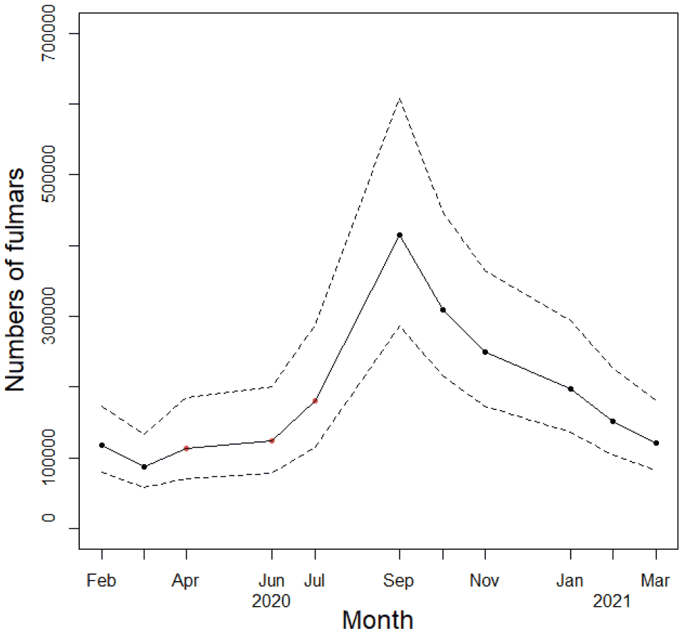
The separate fitted models for breading and non-breeding season are given in Table 8. The estimates of numbers of fulmars during the survey period is given in Figure 4. They indicate peak abundance after the end of the breeding season, in September declining thereafter.
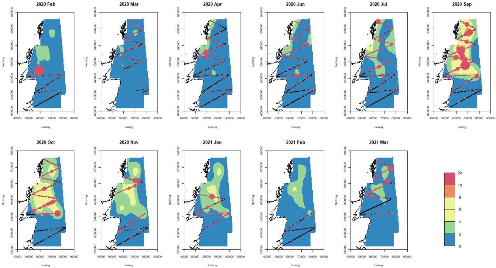
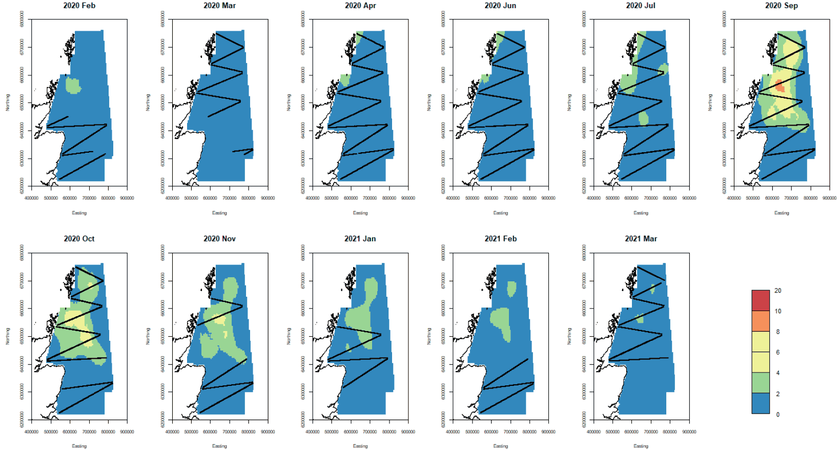
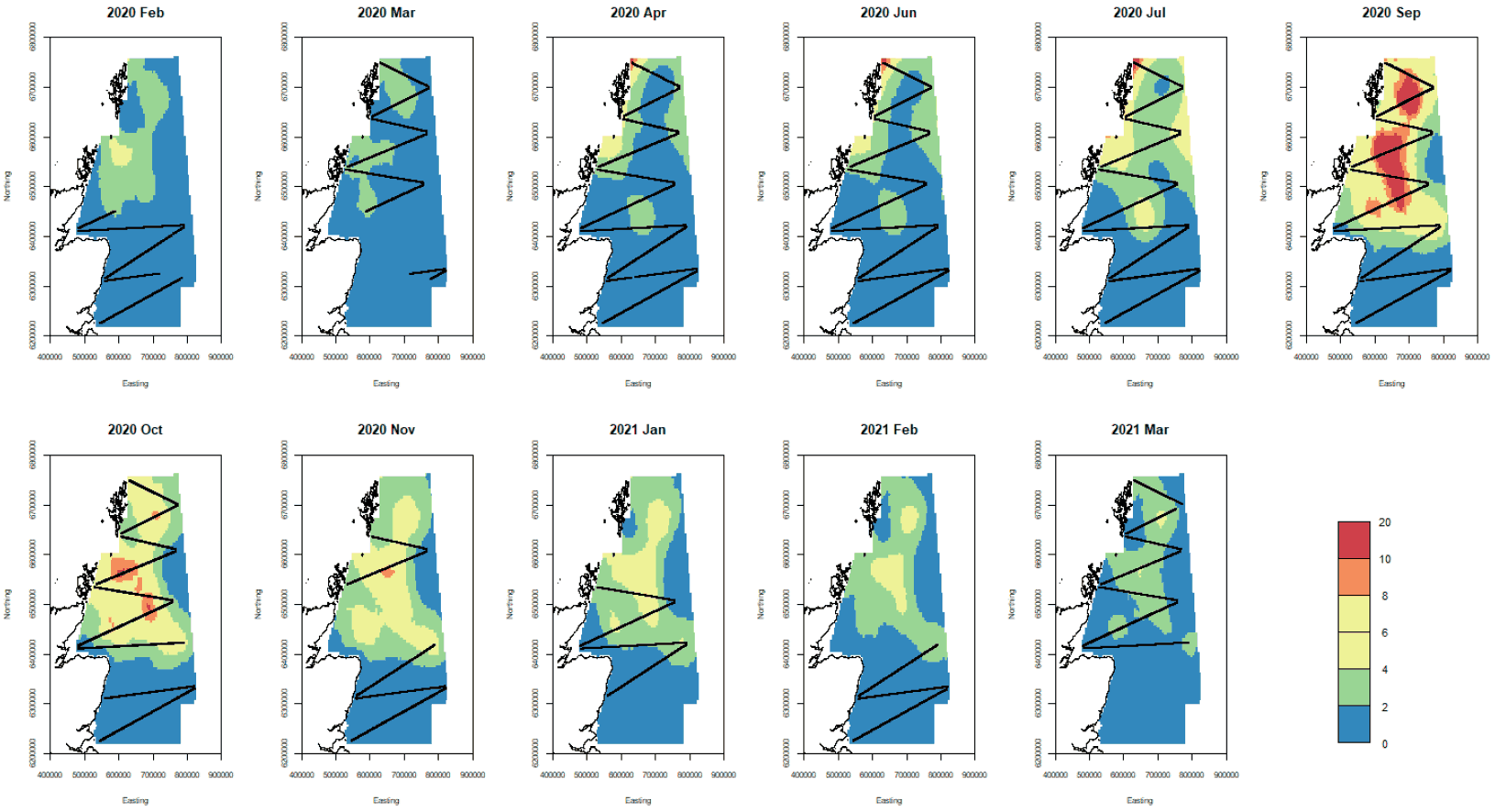
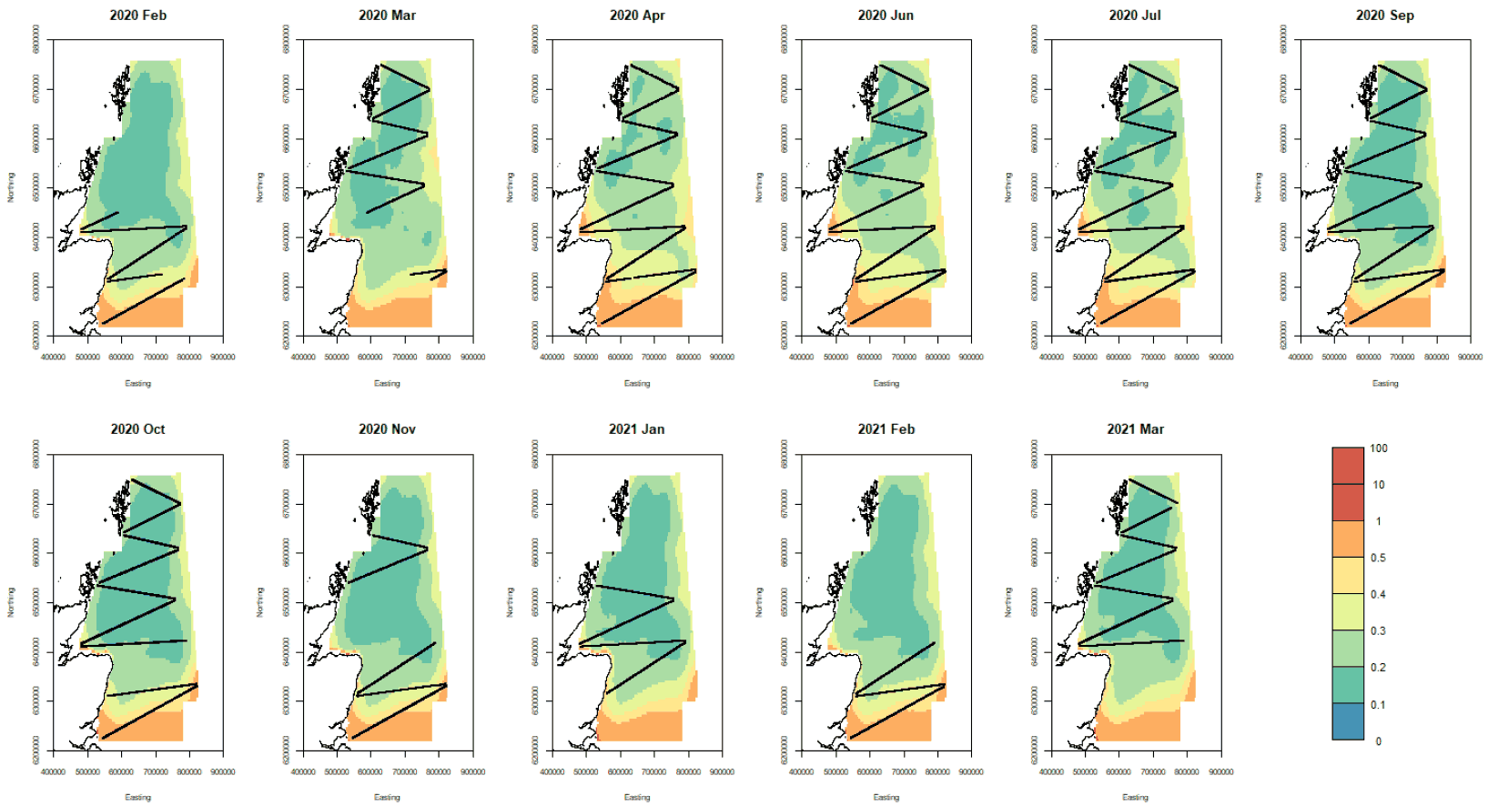
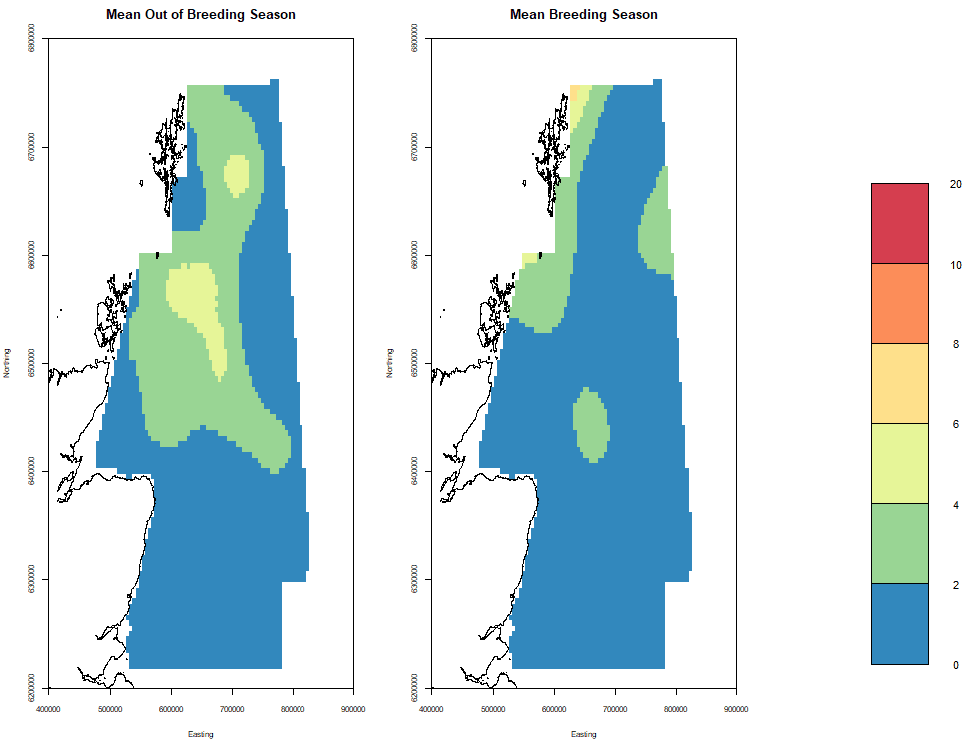
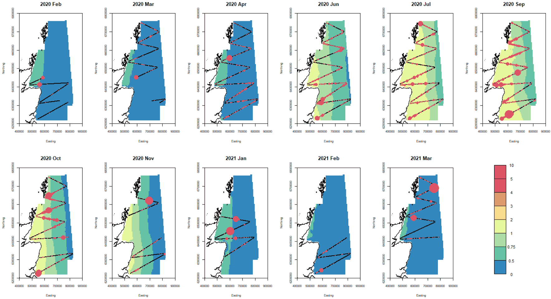
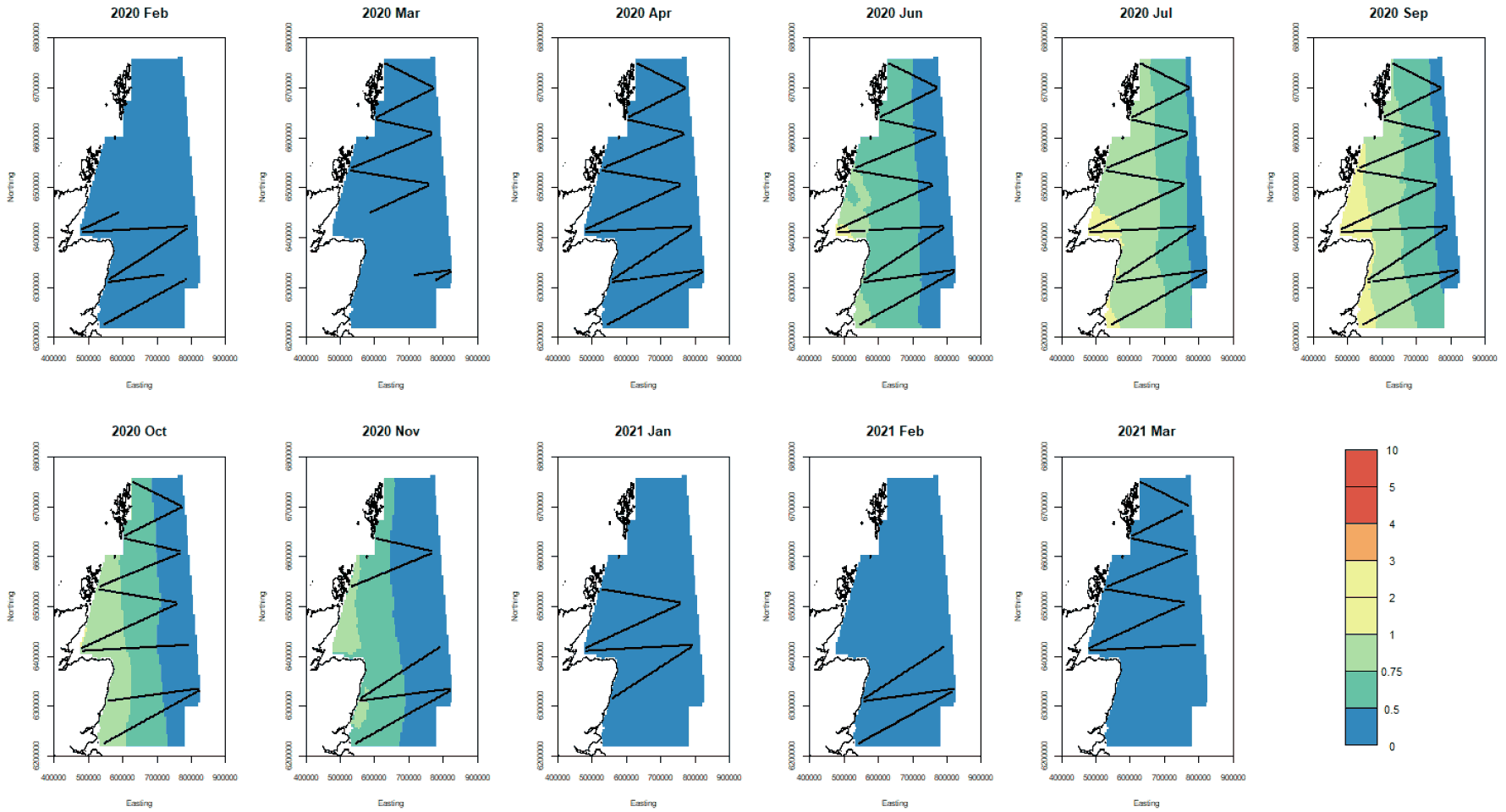
Point estimates of fulmar density for the sampling months along with the confidence bounds are given in Figure 5, Figure 6, and Figure 7. They show highest densities offshore in the northernmost part of the North Sea east of Shetland and Orkney south to the Moray Firth. The CVs are shown in Figure 8 and are largest at the southern areas of the study site. The mean point estimates for breeding and non-breeding season in shown in Figure 9. The breeding distribution is closer to the shore than in the non-breeding season.
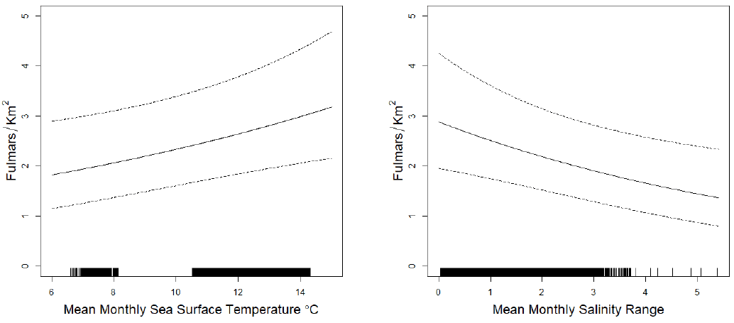
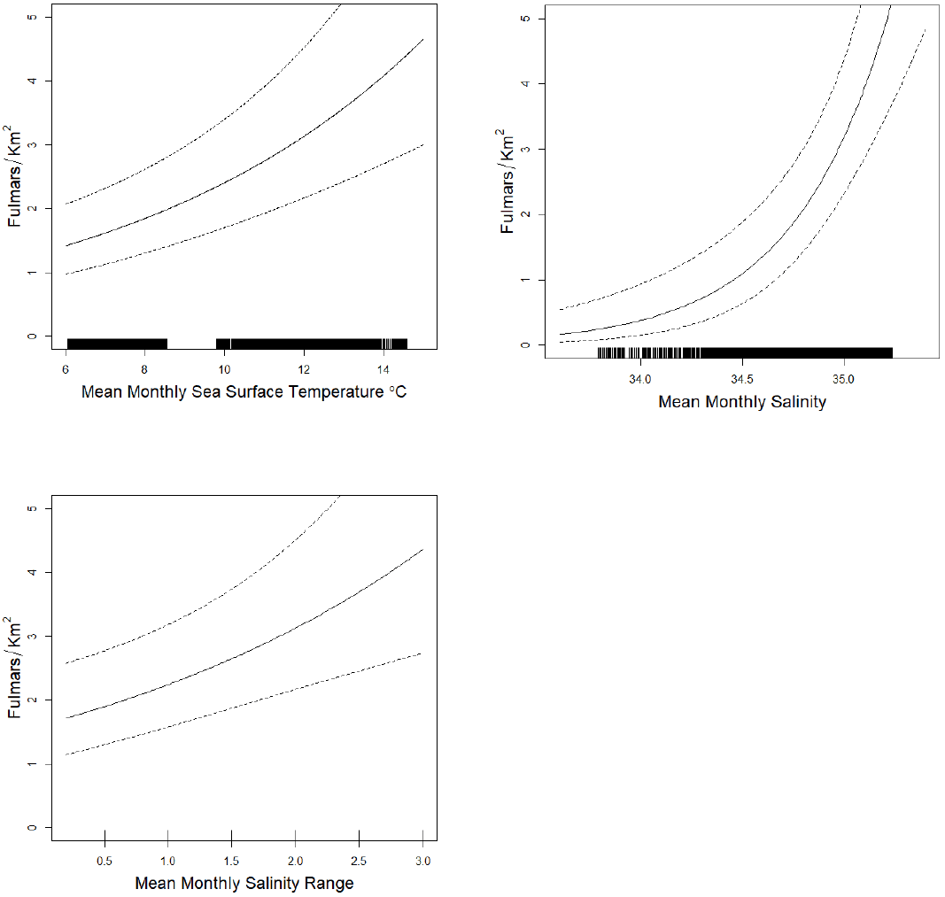
The effect of the non-location variables, sea surface temperature (SST) and salinity, in the breeding season model, is given in Figure 10. They indicate a general increase in fulmar densities with increasing SST and decreasing salinity during this season.
The effect of the same non-location variables as well as salinity range in the non-breeding season model, is given in Figure 11. They showed positive relationships of fulmar density with both SST and salinity during the non-breeding season.
Note that these are the effects of these variables given the presence of location in the model, so they may be very different from the actual biological effect.
6.3.2 Northern Gannet
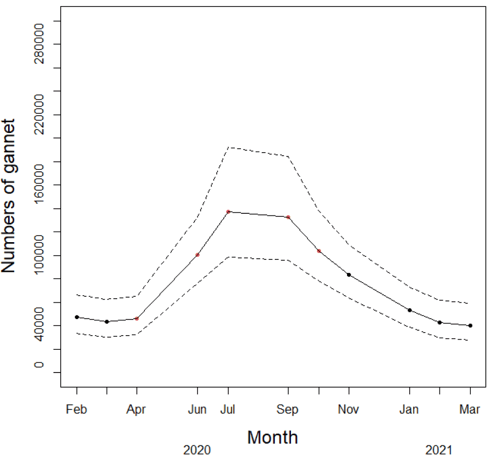
The best fit single model for the whole year is given in Table 8. Estimated numbers during the study period are depicted in Figure 12. They show a strong peak during the main breeding season between June and October.
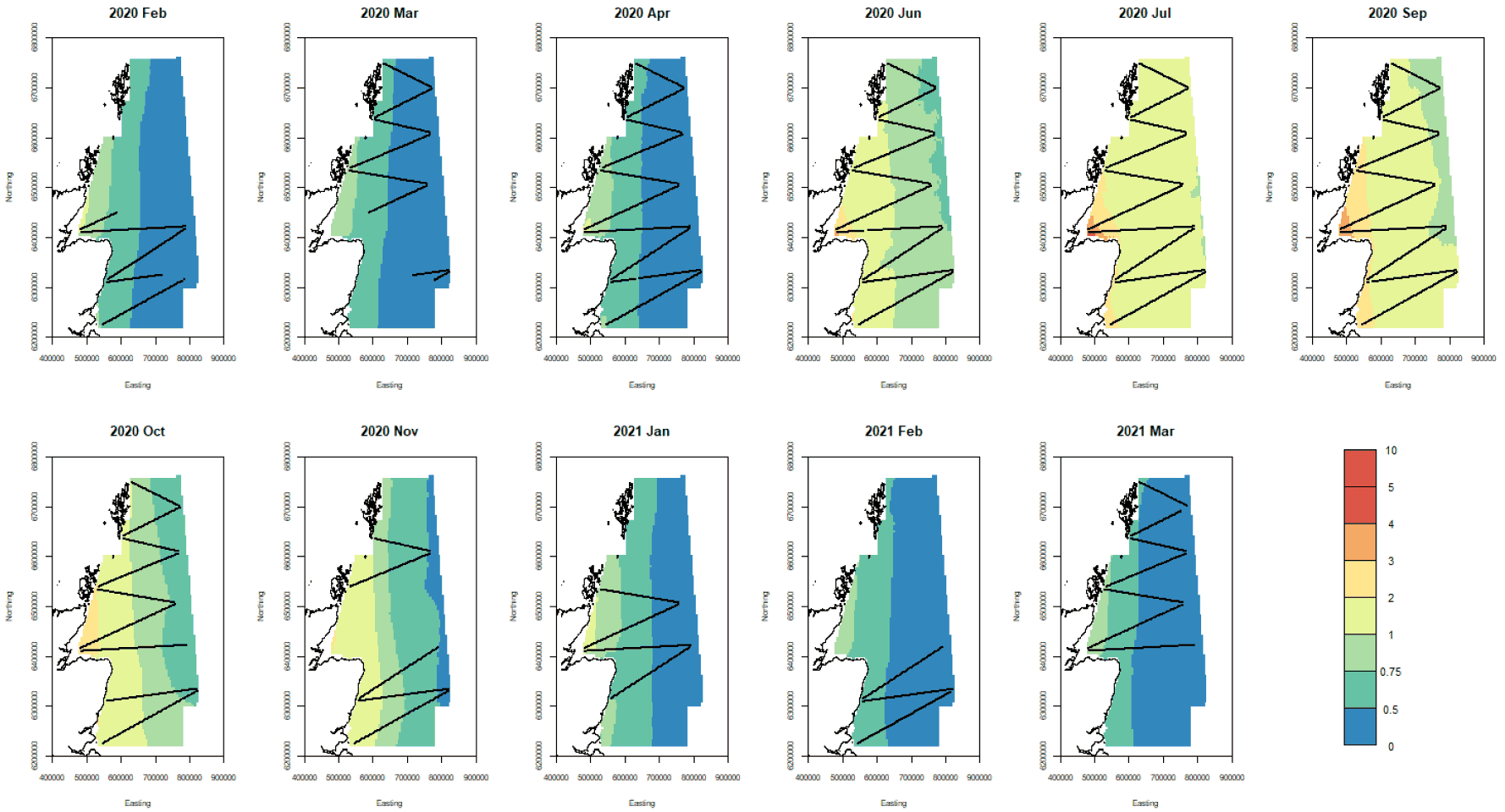
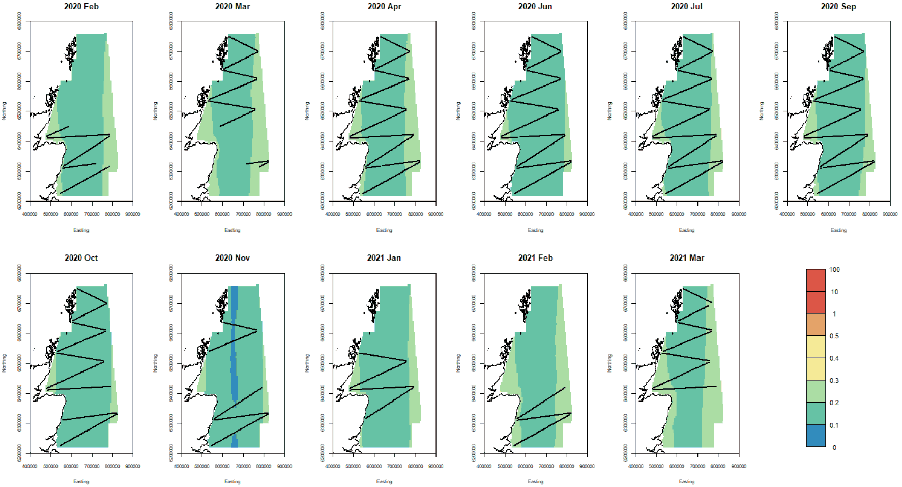
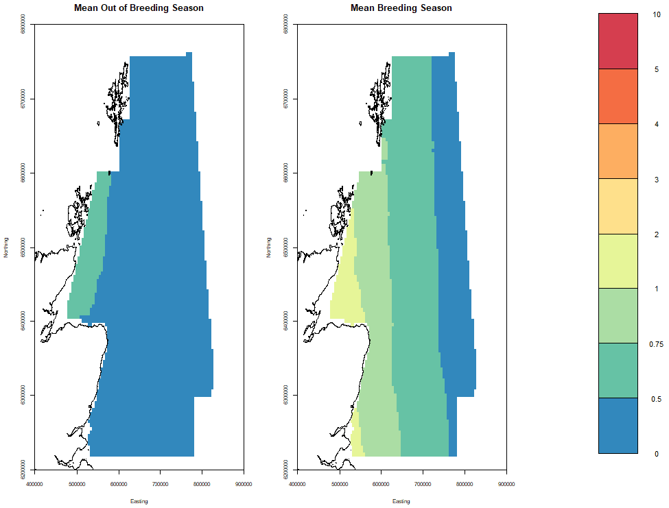
Point estimates of gannet density for the sampling months along with the confidence bounds are given in Figures Figure 13, Figure 14 and Figure 15. They indicate a wide offshore distribution between June and October, with smaller numbers between November and March occurring closer inshore in areas such as the Moray Firth. The CVs are shown in Figure 16 and are largest along the east and west border of the study area. The mean point estimates for breeding and non-breeding season in shown in Figure 17. The breeding distribution of birds is closer to the shore than in the non-breeding season.
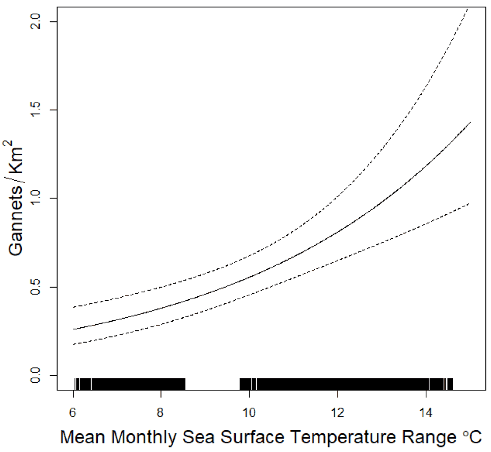
The effect of sea surface temperature range on density is given in Figure 18, and shows a general positive trend.
6.3.3 Great Skua
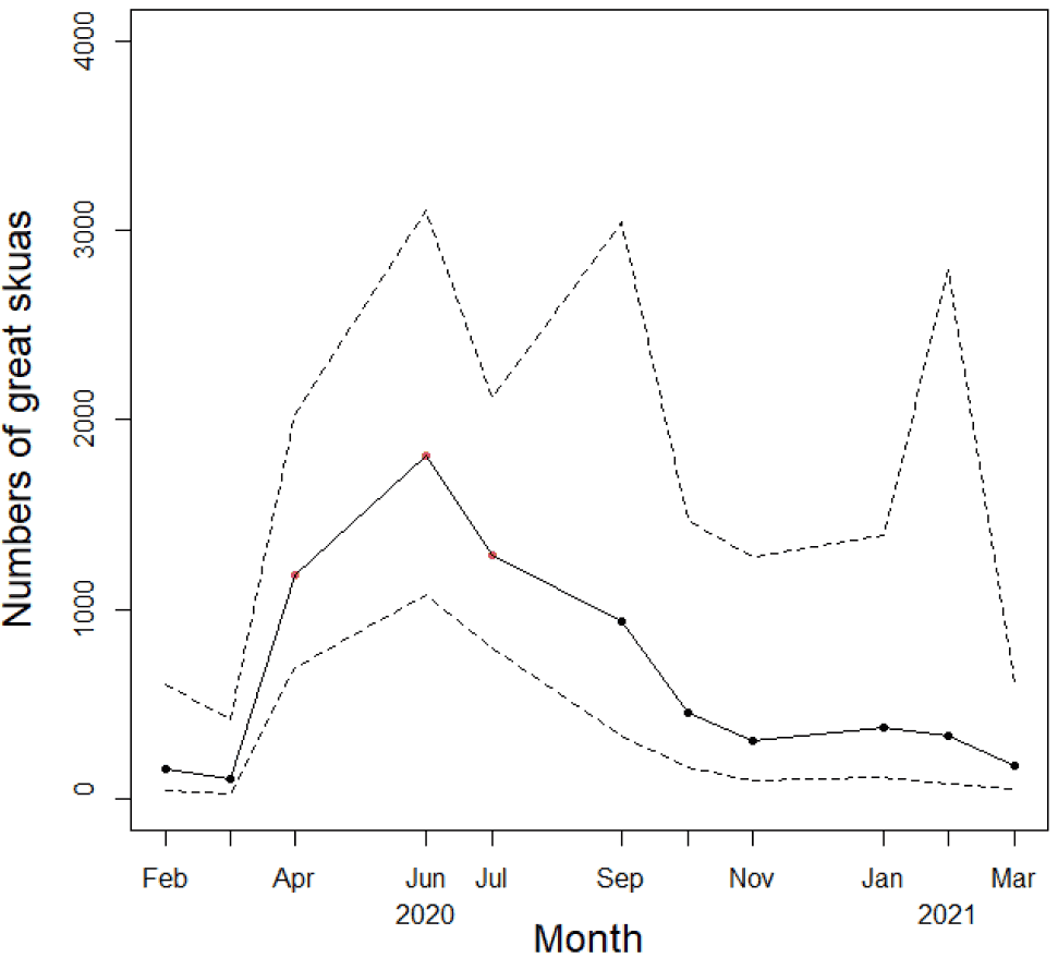
The model based on the amalgamated data set is given in Table 8. The estimates of numbers of great skuas during the survey period is given in Figure 19. They indicate peak abundance during the breeding season. The results of this model should be treated with caution as the diagnostics of the model were not ideal.
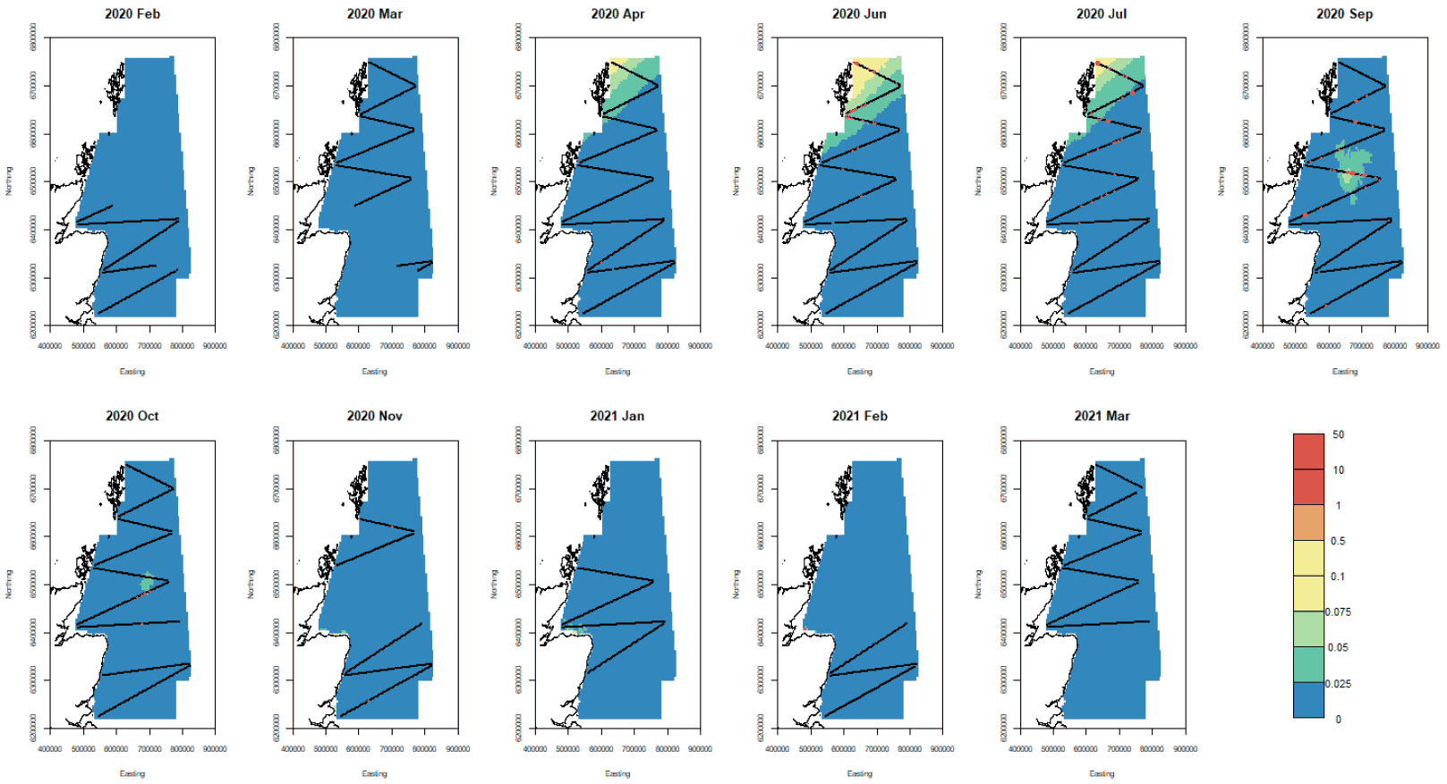
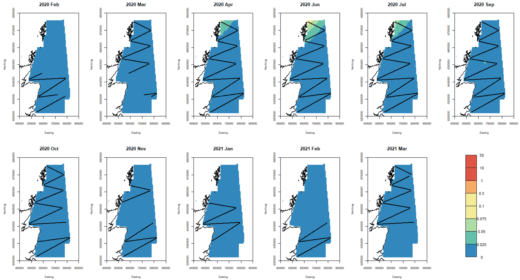
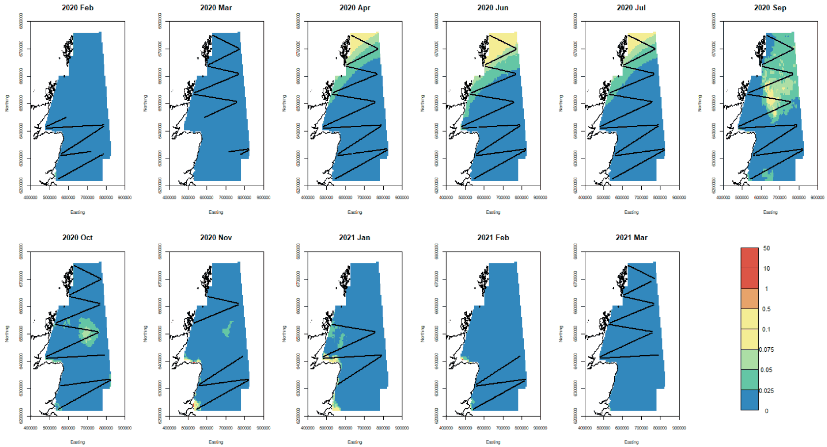
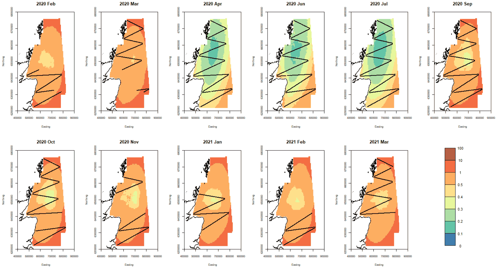
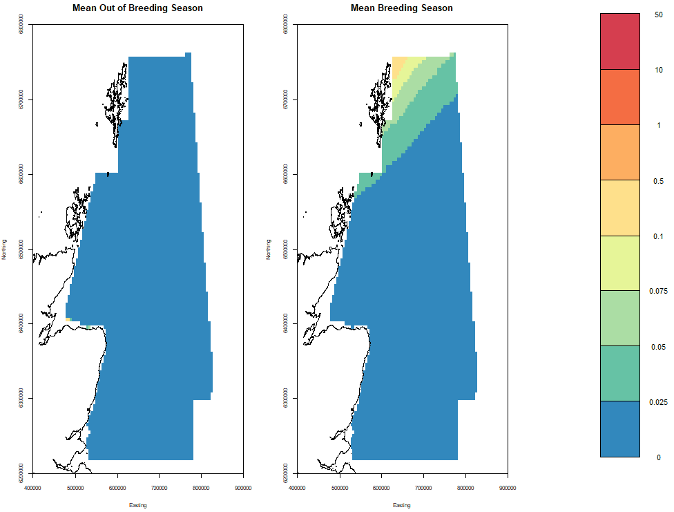
Point estimates of great skua density for the sampling months along with the confidence bounds are given in Figures Figure 20, Figure 21 and Figure 22. They show highest densities in the far north-western part of the survey region east of Shetland. The CVs are shown in Figure 23 and are largest at the southern areas of the study site during the breeding season and at the peripheral areas of the study site outside the breeding season. The mean point estimates for breeding and non-breeding season in shown in Figure 24 The breeding distribution is concentrated at the northern site of the study area.
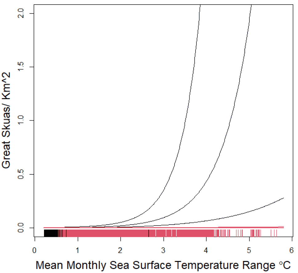
The effect of the non-location variable, sea surface temperature monthly range, in (red) and outside (black) the breeding season, is given in Figure 25.
Note that these are the effects given the presence of location in the model, so they may be very different from the actual biological effect.
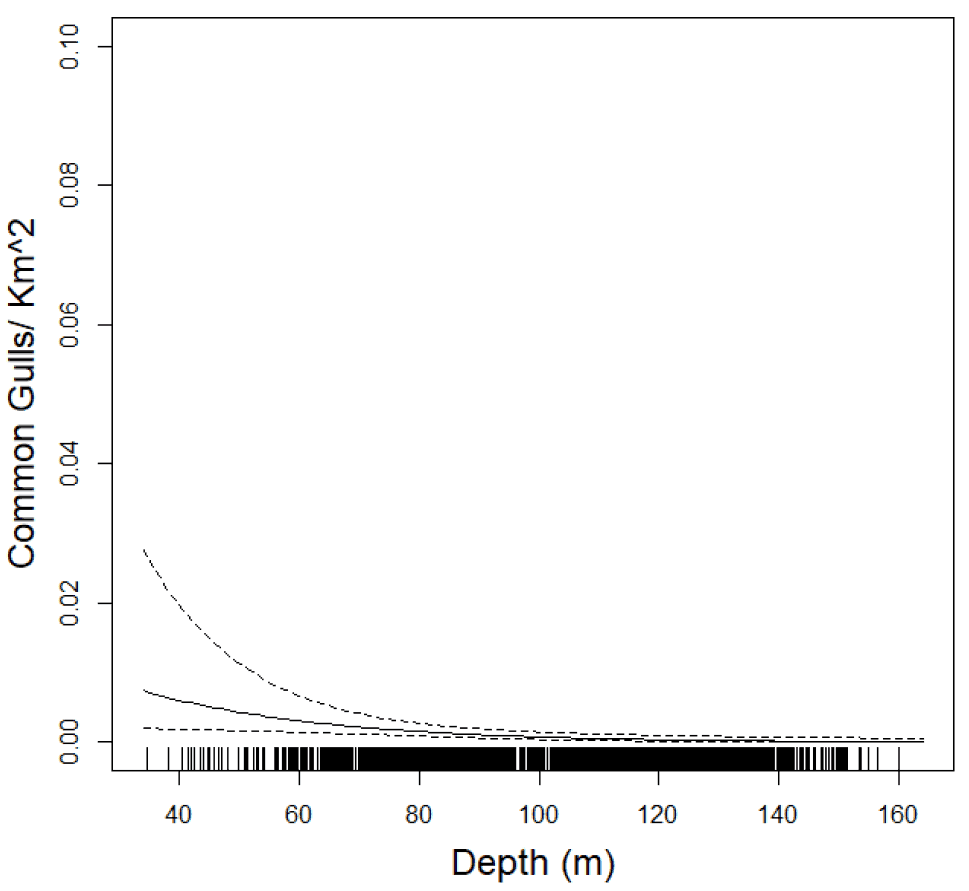
6.3.4 Common Gull
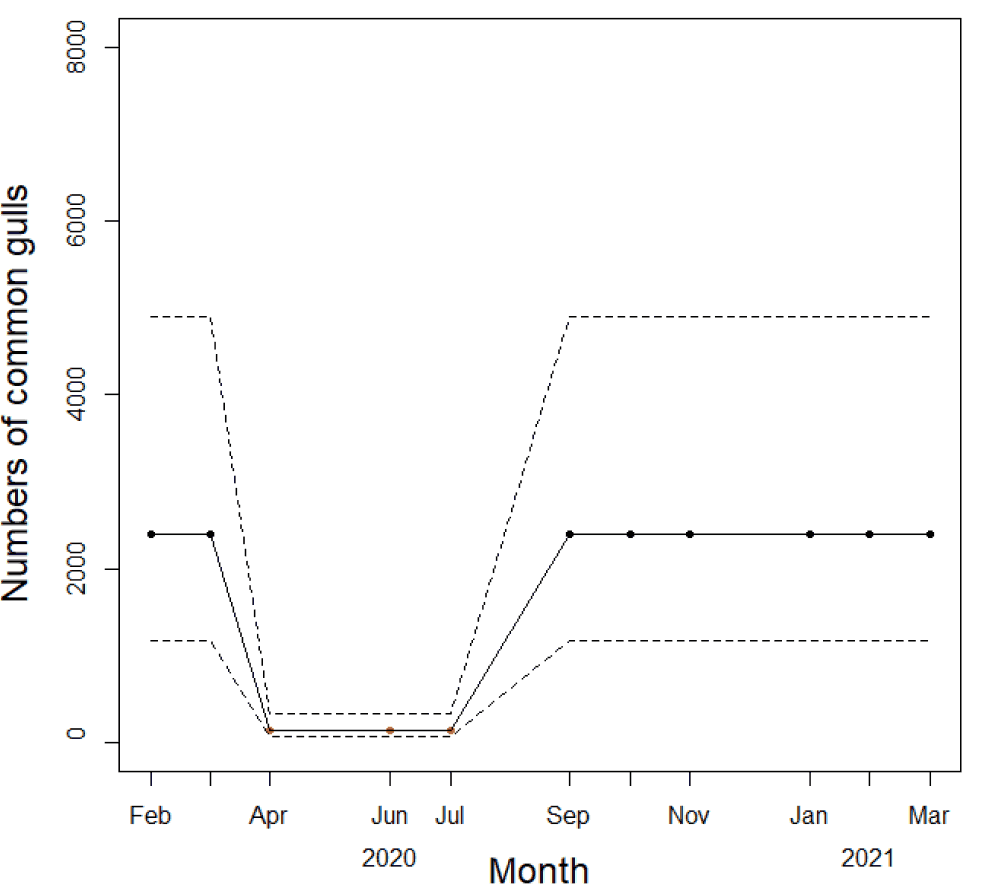
Predictions based a breeding season model is given in Table 8. No model was fitted to non-breeding season. Estimates of numbers in the area over the survey period are given in Figure 26. They show a general increase in abundance in the study area in the autumn. Results are constant within season.
Point estimates of common gull density for the sampling months along with the confidence bounds are given in Figure 27, Figure 28, and Figure 29. They indicate higher densities mainly off the coast during the breeding season. As the spatial pattern was uniform and consistent over the survey month for both breeding and non-breeding season, seasonal spatial patterns are not presented for this species as it can be deduced from Figure 27, Figure 28, Figure 29. The CVs are shown in Figure 30 and are largest at the central and norther part of the study site.
The effect of depth during the breeding season is shown in Figure 31.
6.3.5 Lesser Black-backed Gull
No variables were found that could predict the density of lesser black-backed gulls when the autocorrelation in the data was considered. The best estimate for abundance was 640 (95% CI: 280-1490). This species was only observed during five surveys and in very low numbers.
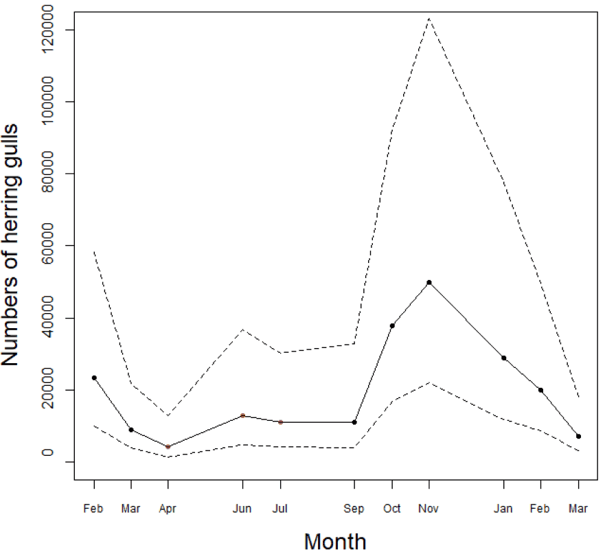
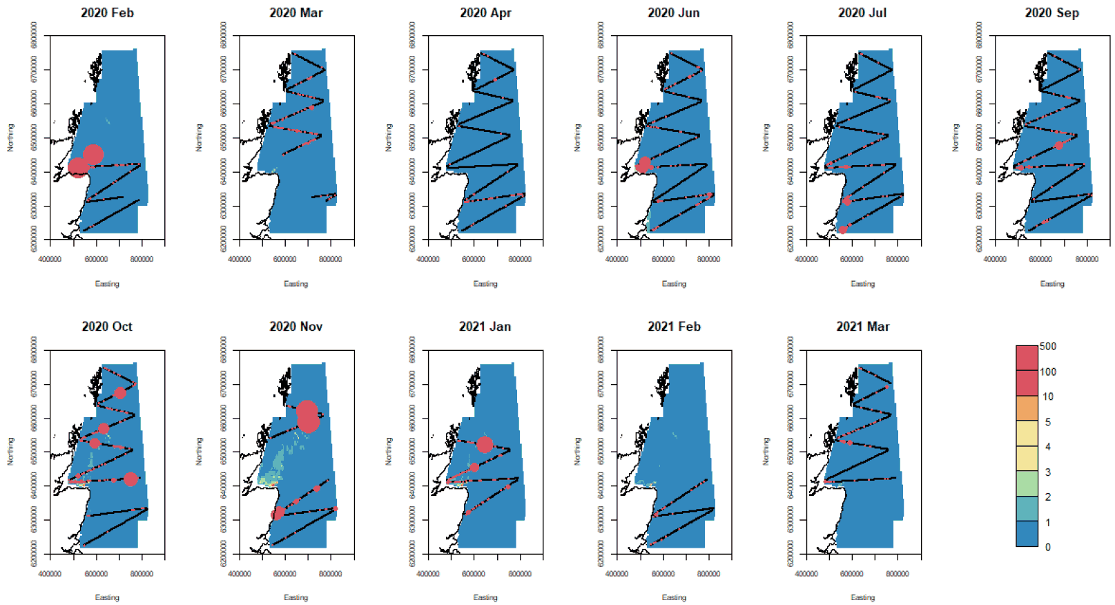
6.3.6 Herring Gull
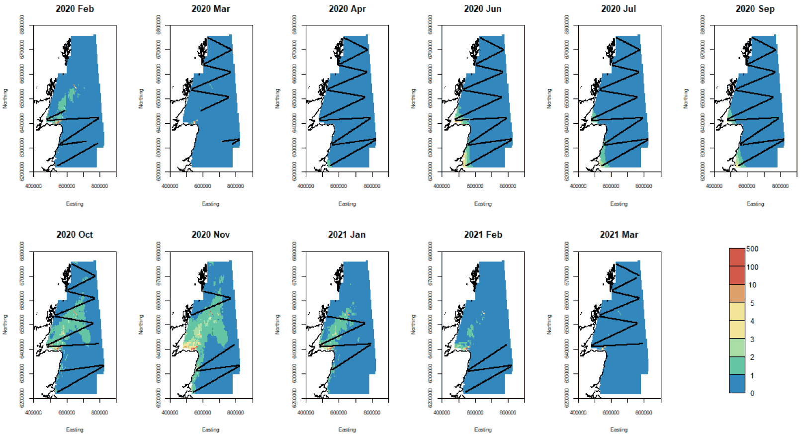
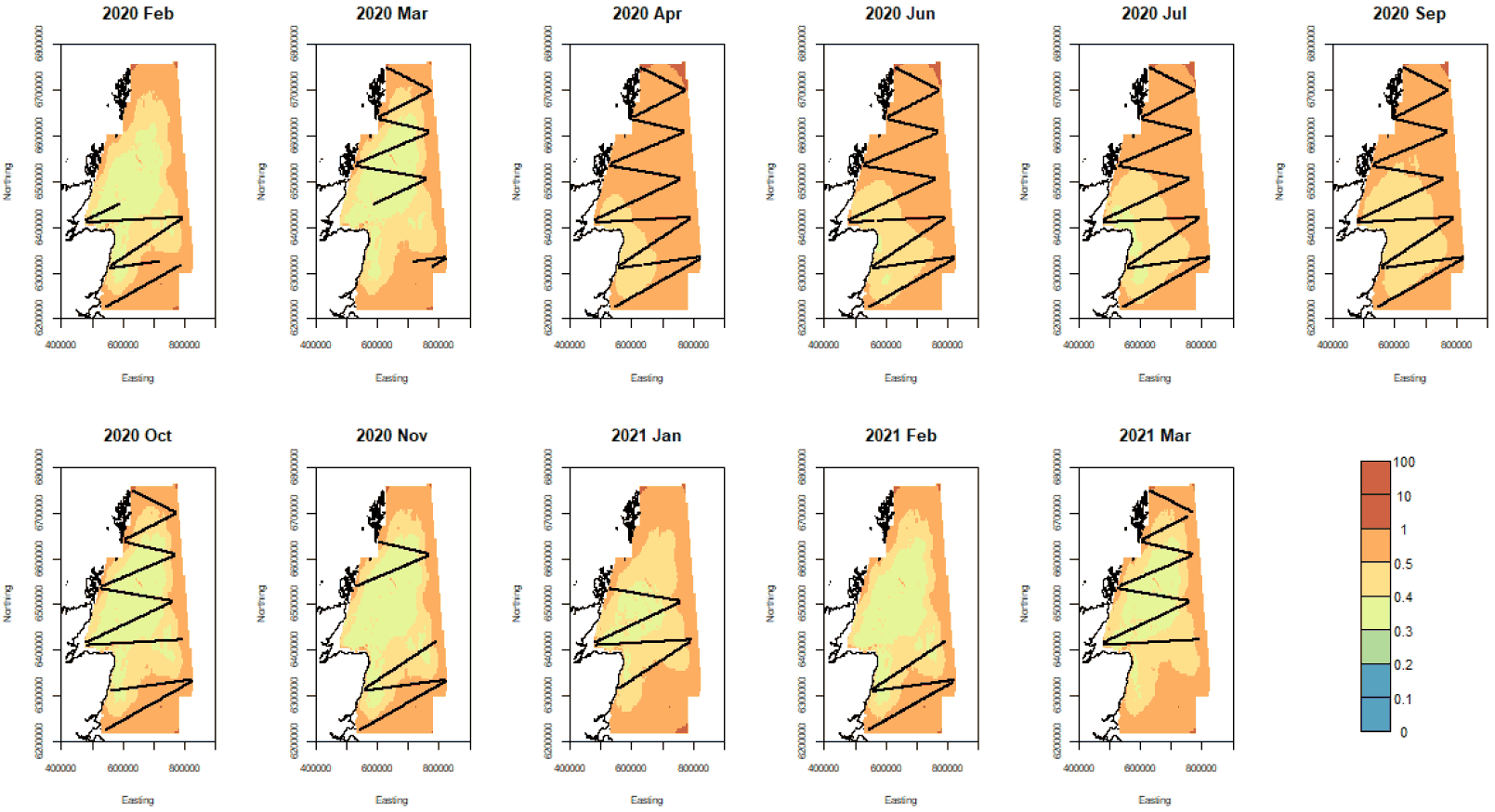
The single (all year) fitted model is given in Table 8. Estimates of numbers in the area over the survey period are given in Figure 32. They show a general increase in abundance in the study area between September and March.
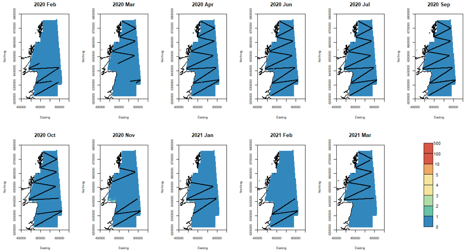
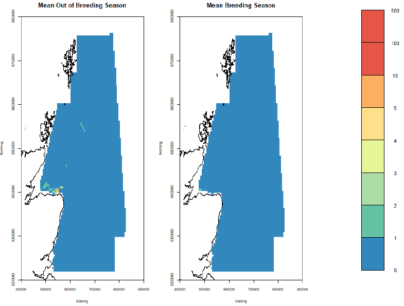
Point estimates of herring gull density for the sampling months along with the confidence bounds are given in Figure 33, Figure 34, and Figure 35. They indicate higher densities in the vicinity of the Moray Firth in October and November. The CVs are shown in Figure 36 and are largest at the peripheries of the study area. The mean point estimates for breeding and non-breeding season in shown in
Figure 37. The breeding distribution is closer to the shore in the non-breeding season.
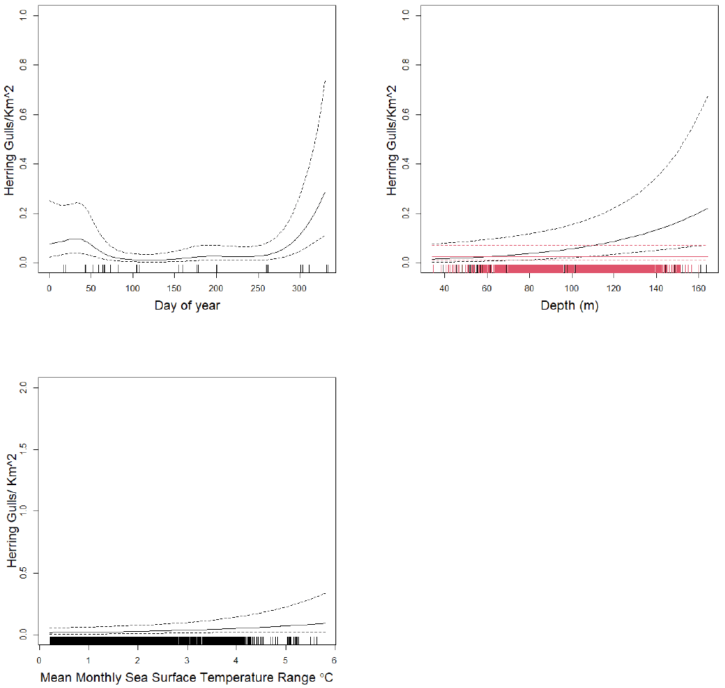
The non-location spatial effects in all year model for herring gull are given below. They show greater densities in winter, and at greater depths during the breeding season but no relationship in the non-breeding season (Figure 38).
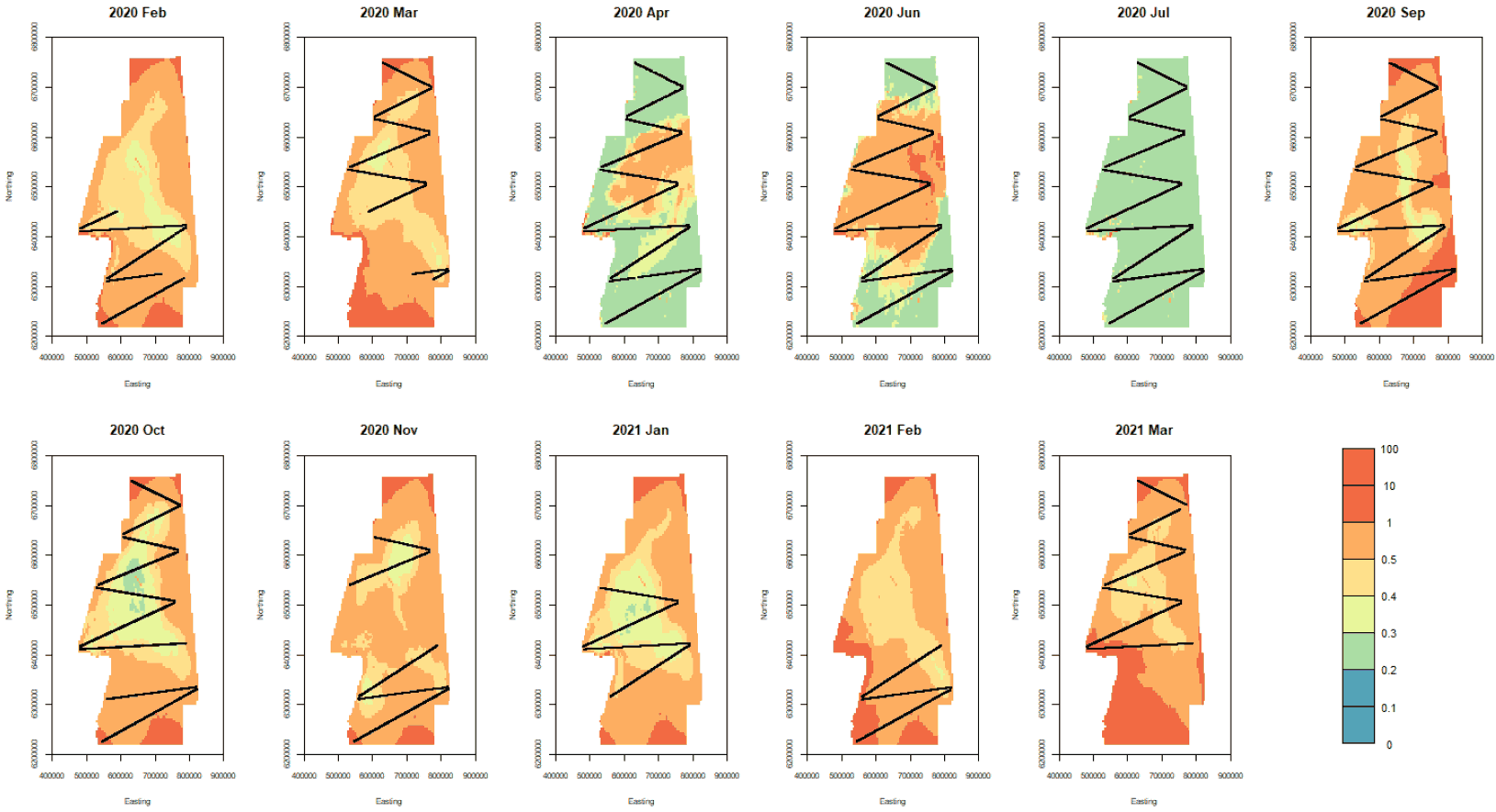
6.3.7 Great Black-backed Gull
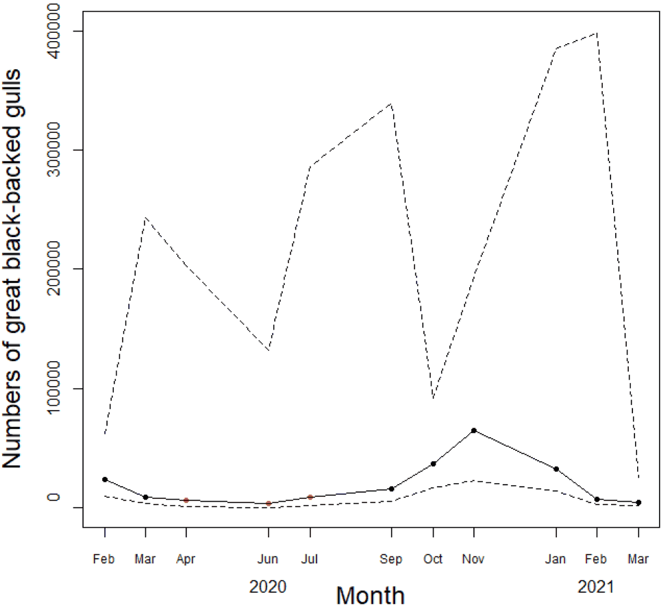
The separate fitted models for the breading and non-breeding season are given in Table 8. Estimated numbers through the study period are shown in Figure 39 and indicate relatively low numbers throughout the year but with a small peak between October and January.
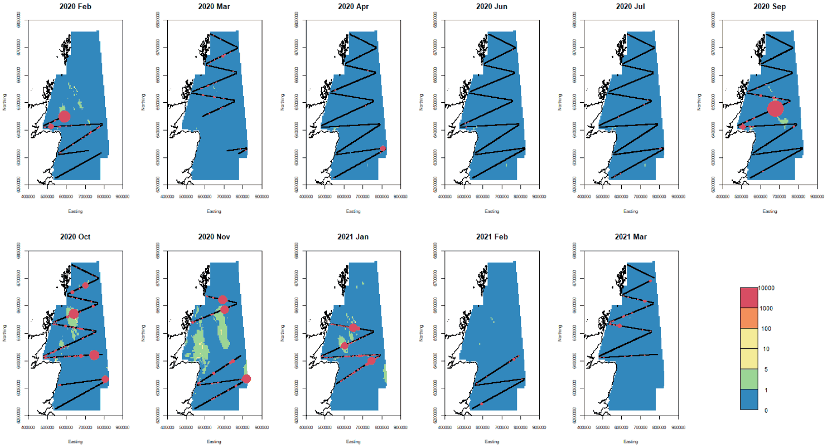
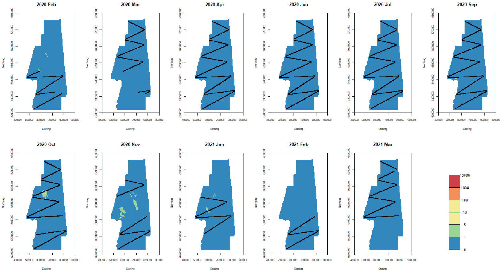
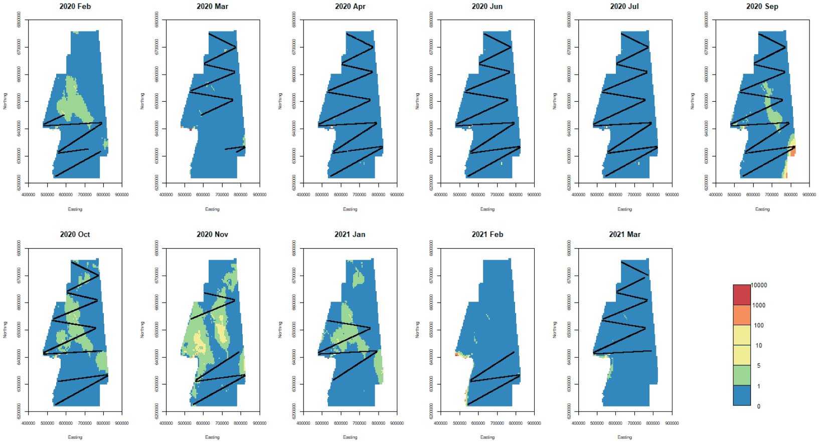
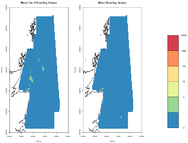
Point estimates of gull density for the sampling months along with the confidence bounds are given in Figure 40, Figure 41, and Figure 42. There is high uncertainty in some peripheral regions of the survey region leading to the high upper bounds in Figure 42. Areas with higher densities occur east of Orkney and around the Moray Firth between October and February. The CVs are shown in Figure 43 and are largest at the southern areas of the study site outside the breeding season and in the centre of the study area during the breeding season. The mean point estimates for breeding and non-breeding season in shown in Figure 44. The breeding distribution is further off shore than in the breeding season.
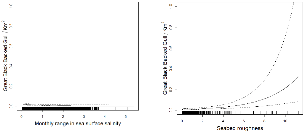
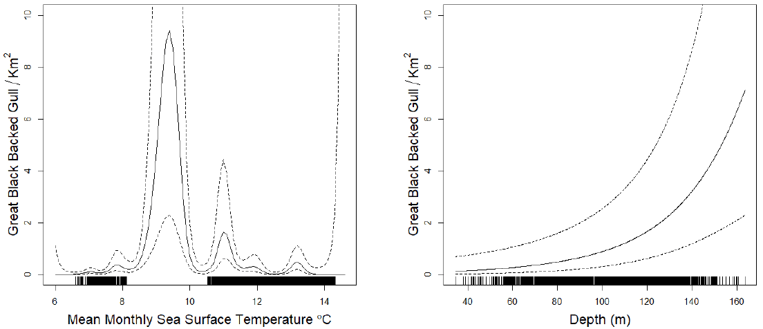
The effect of salinity and seabed roughness in the breeding season model is given in Figure 45. Any salinity effect is weak compared to the effect of greatest seabed roughness. The effect of depth in the non-breeding season model is given in Figure 46 and shows higher densities at greater depths. The relationship with sea surface temperature is difficult to interpret and the model is quite possibly overfitting.
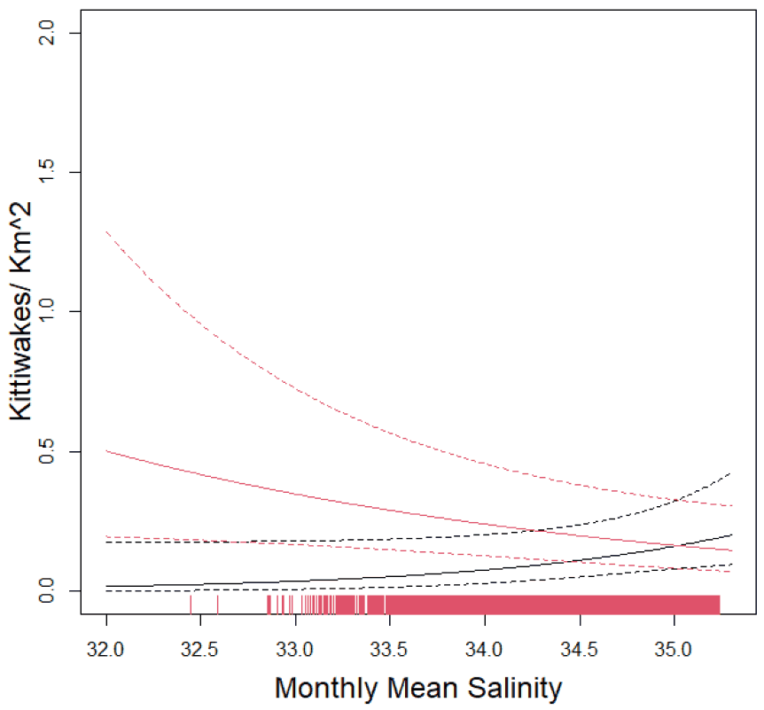
6.3.8 Black-legged Kittiwake
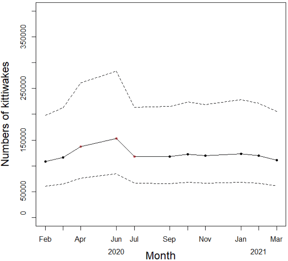
The model for black-legged kittiwakes is given in Table 8. Estimated abundances of kittiwakes through the study period are given in Figure 47. They show a slight increase during the breeding season (April to July) but little change outside that period.
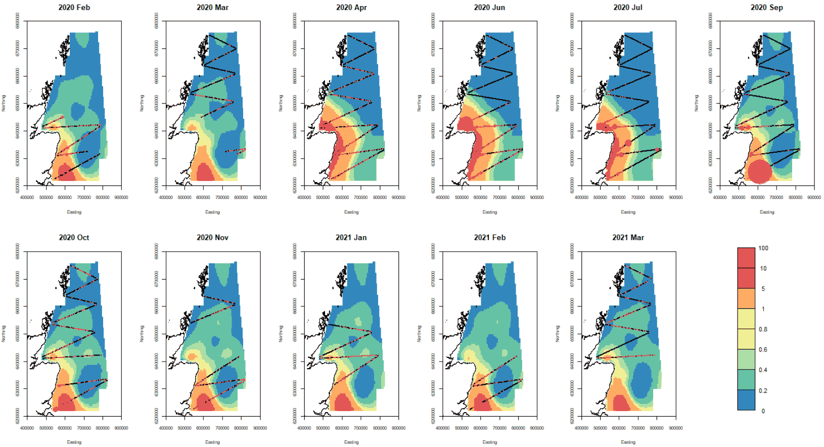
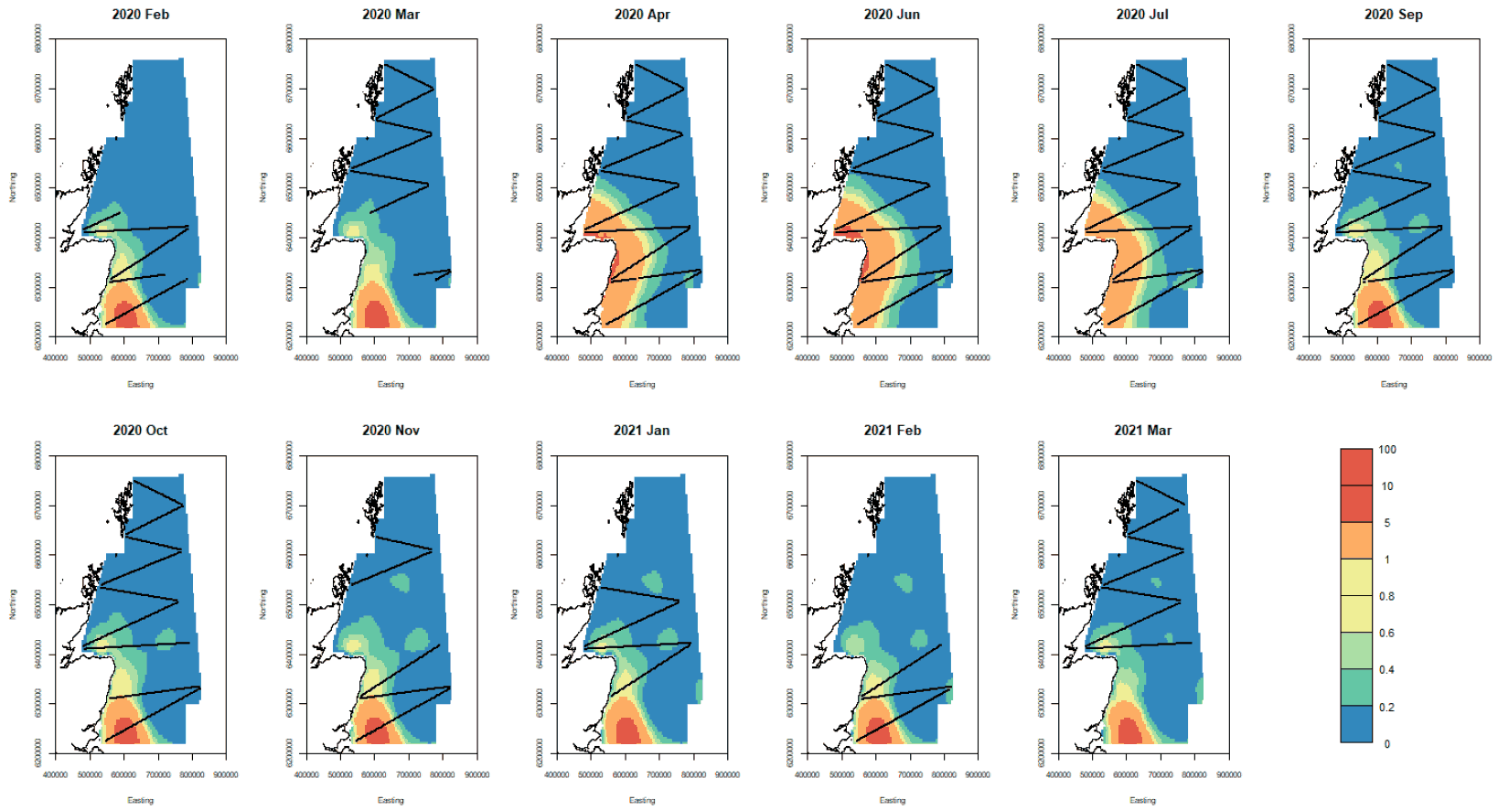
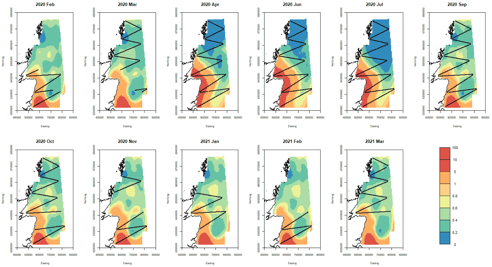
Point estimates of kittiwake density for the sampling months along with the confidence bounds are given in Figure 48, Figure 49, and Figure 50. They indicate greatest densities nearer to the coast around the Moray Firth and Firth of Forth. The CVs are shown in Figure 51 and are largest at the peripheries of the study site. The mean point estimates for breeding and non-breeding season in shown in Figure 52 and is comparable for these two seasons with highest estimates at the south-western part of the study area.
The effect of monthly mean salinity on kittiwake density is shown in Figure 53 and shows opposite trend for breeding (red) and non-breeding season (black) with increase in kittiwake density with decrease in salinity during the breeding season.
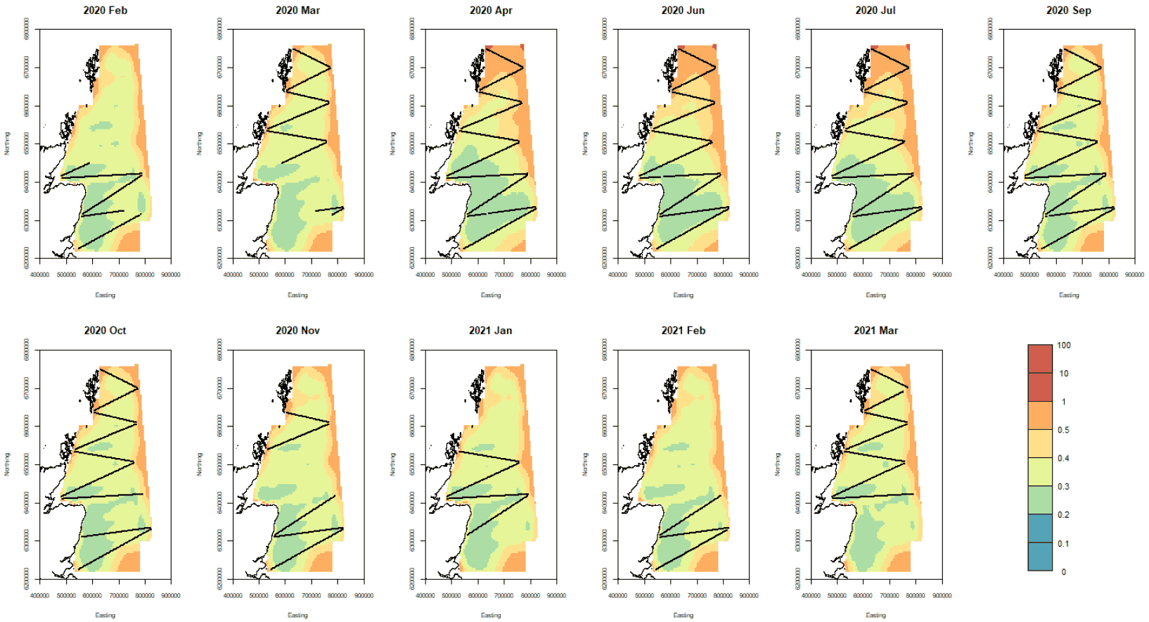
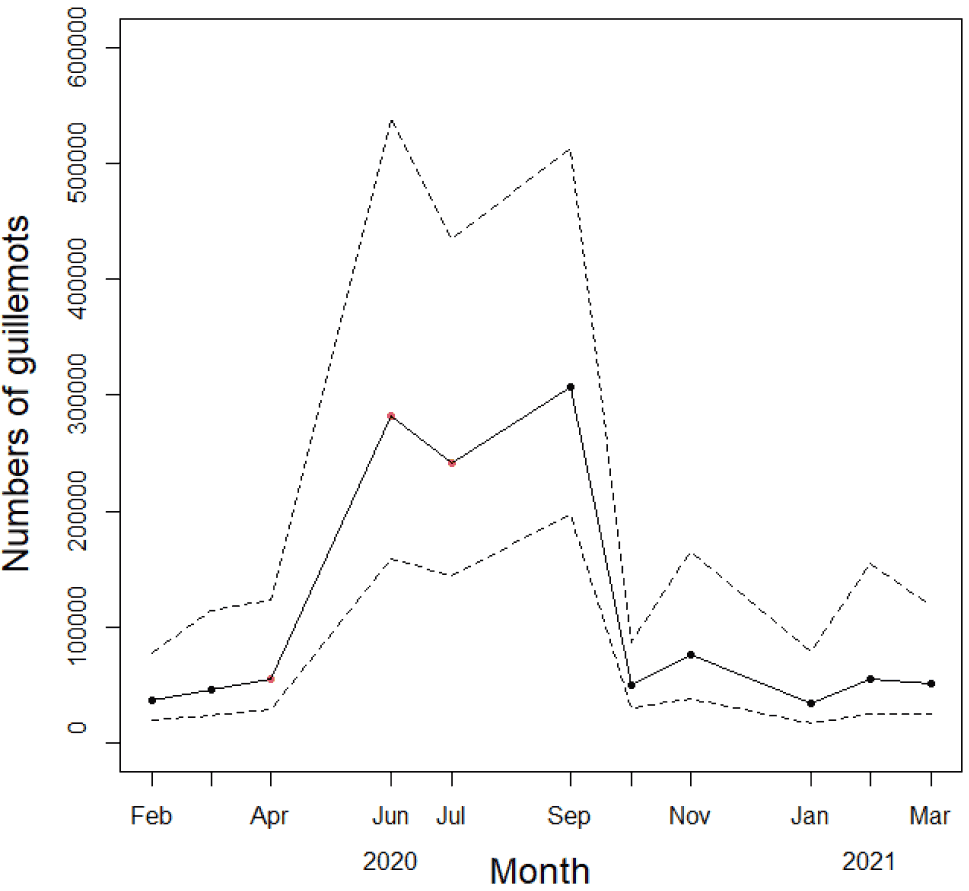
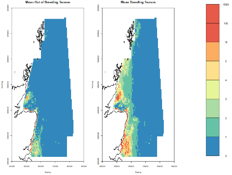
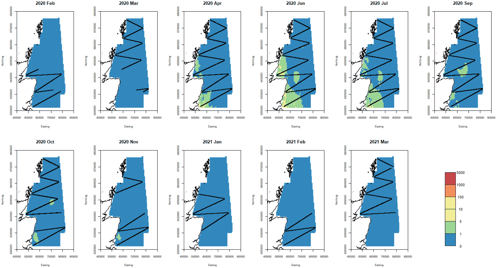
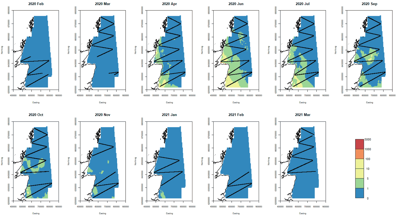
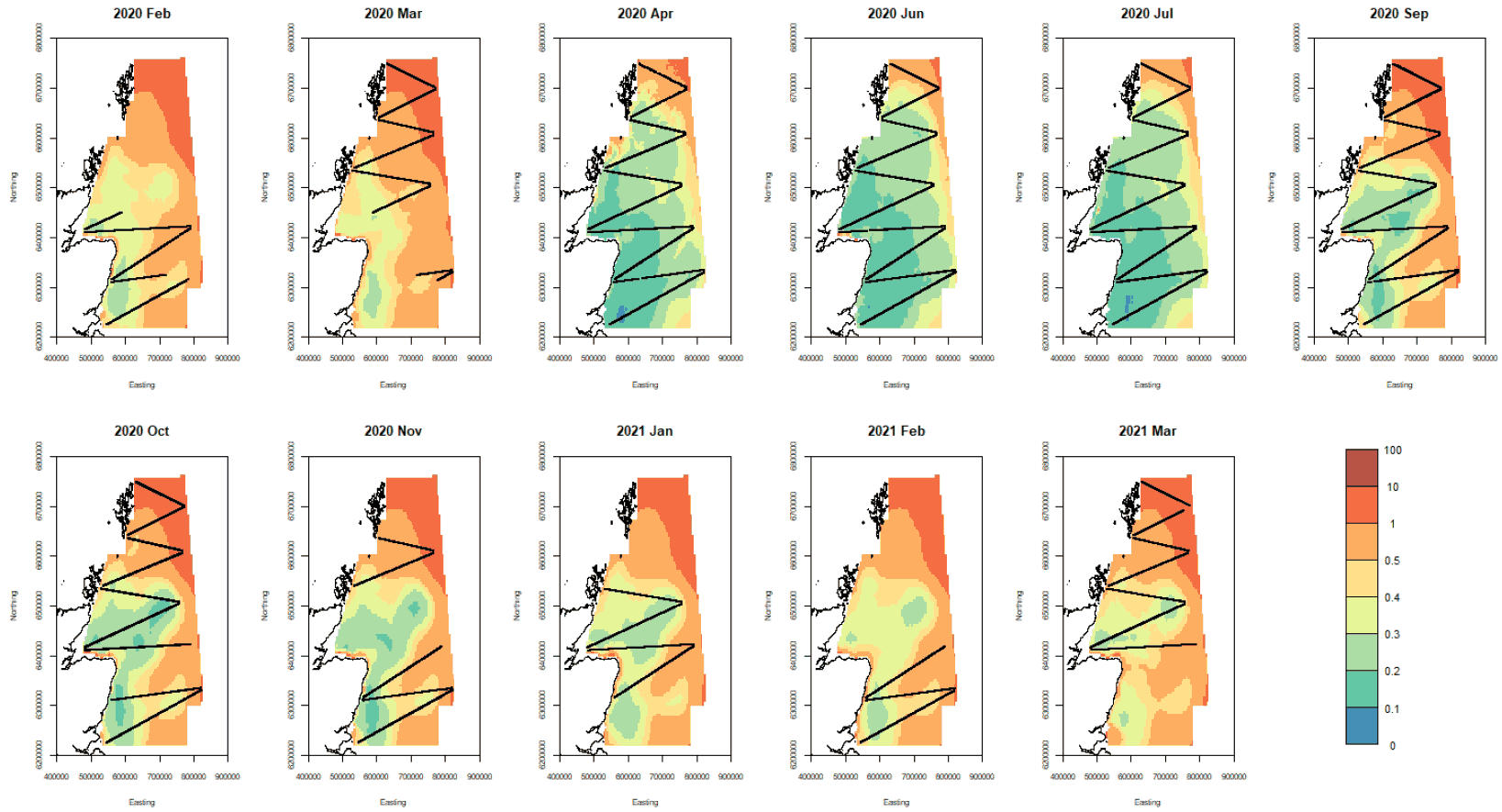
6.3.9 Common Guillemot
The single model (i.e. for the full sampling period) based on the amalgamated data is given in Table 8. The predicted numbers over the period of the survey are given in Figure 54. No stable model with a location effect could be found so the model consisted of main environmental effects only.
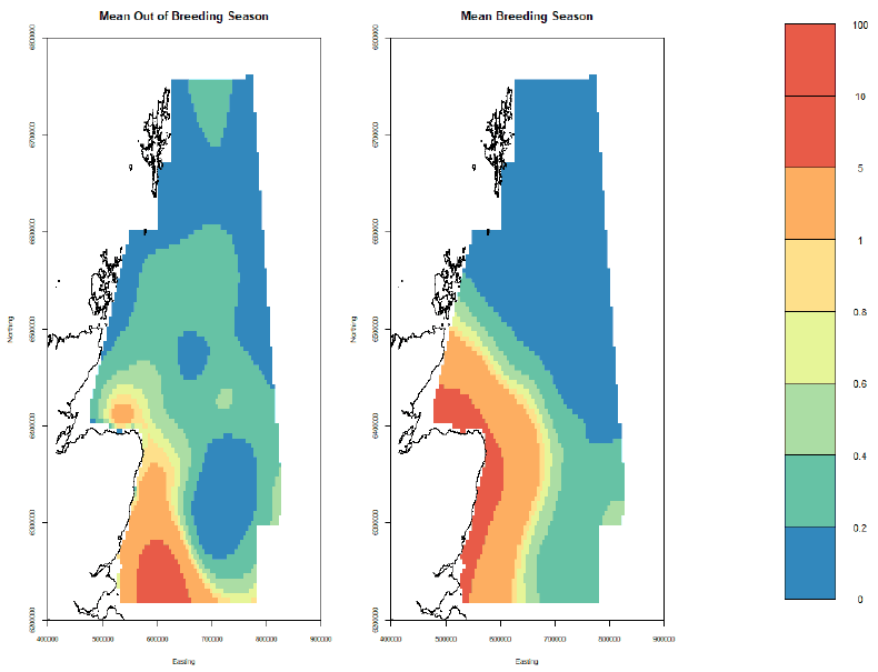
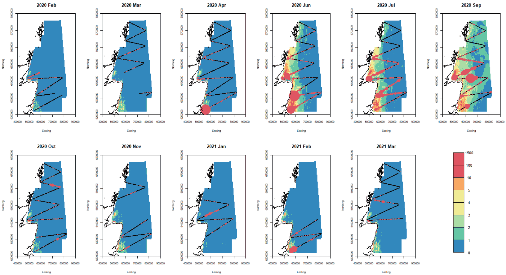
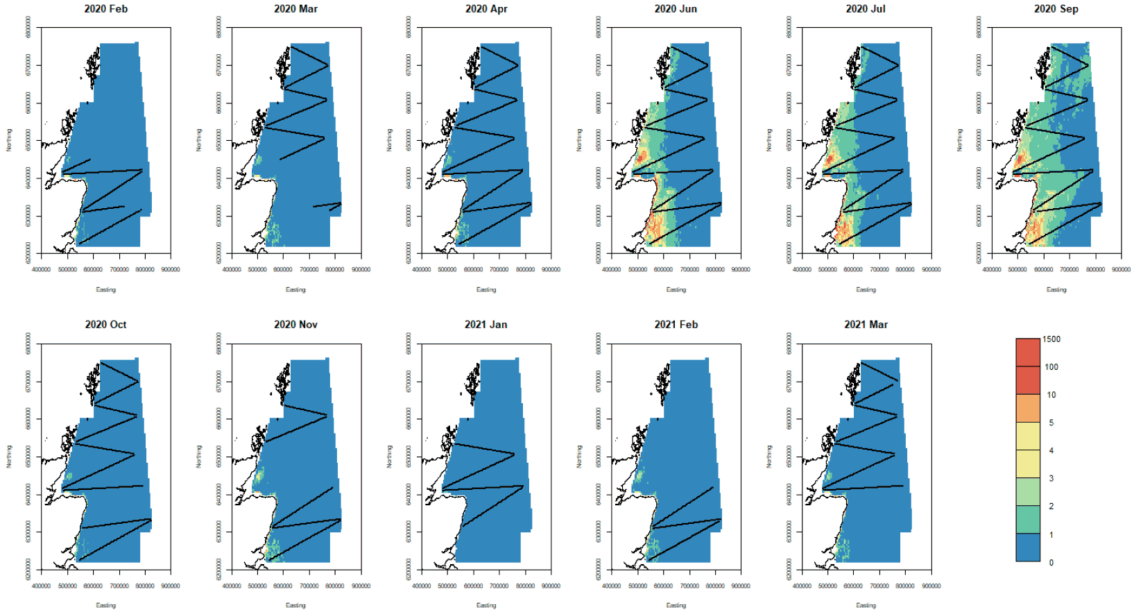
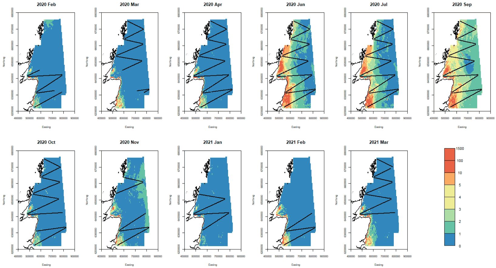
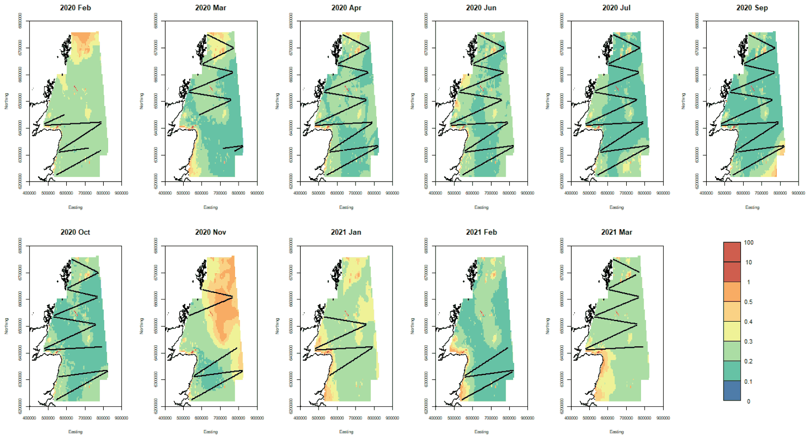
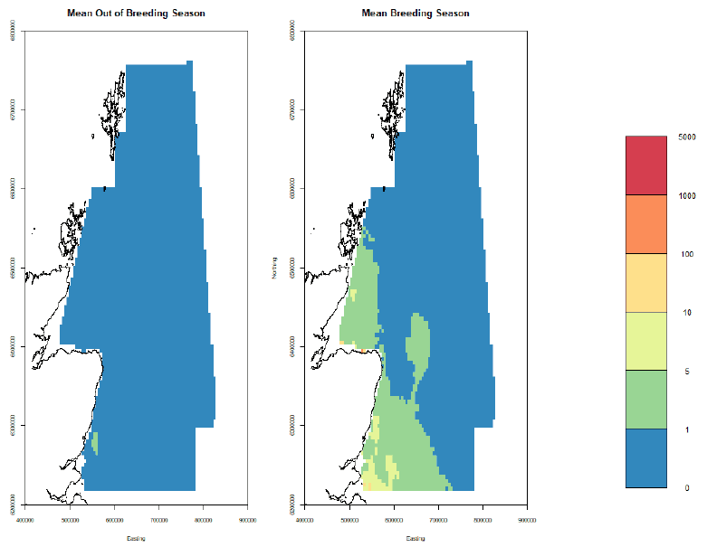
Point estimates of common guillemot density for the sampling months along with the associated confidence bounds are given in Figure 55, Figure 56, and Figure 57. They show greatest densities nearer to the coast in all months, but particularly between June and September from east of Orkney to the Moray Firth, and down the East Grampian coast as far as the Firth of Forth. The CVs are shown in Figure 58 and are largest at different locations over the study period. The mean point estimates for breeding and non-breeding season in shown in Figure 58. The breeding distribution is closer to the shore than in the non-breeding season.
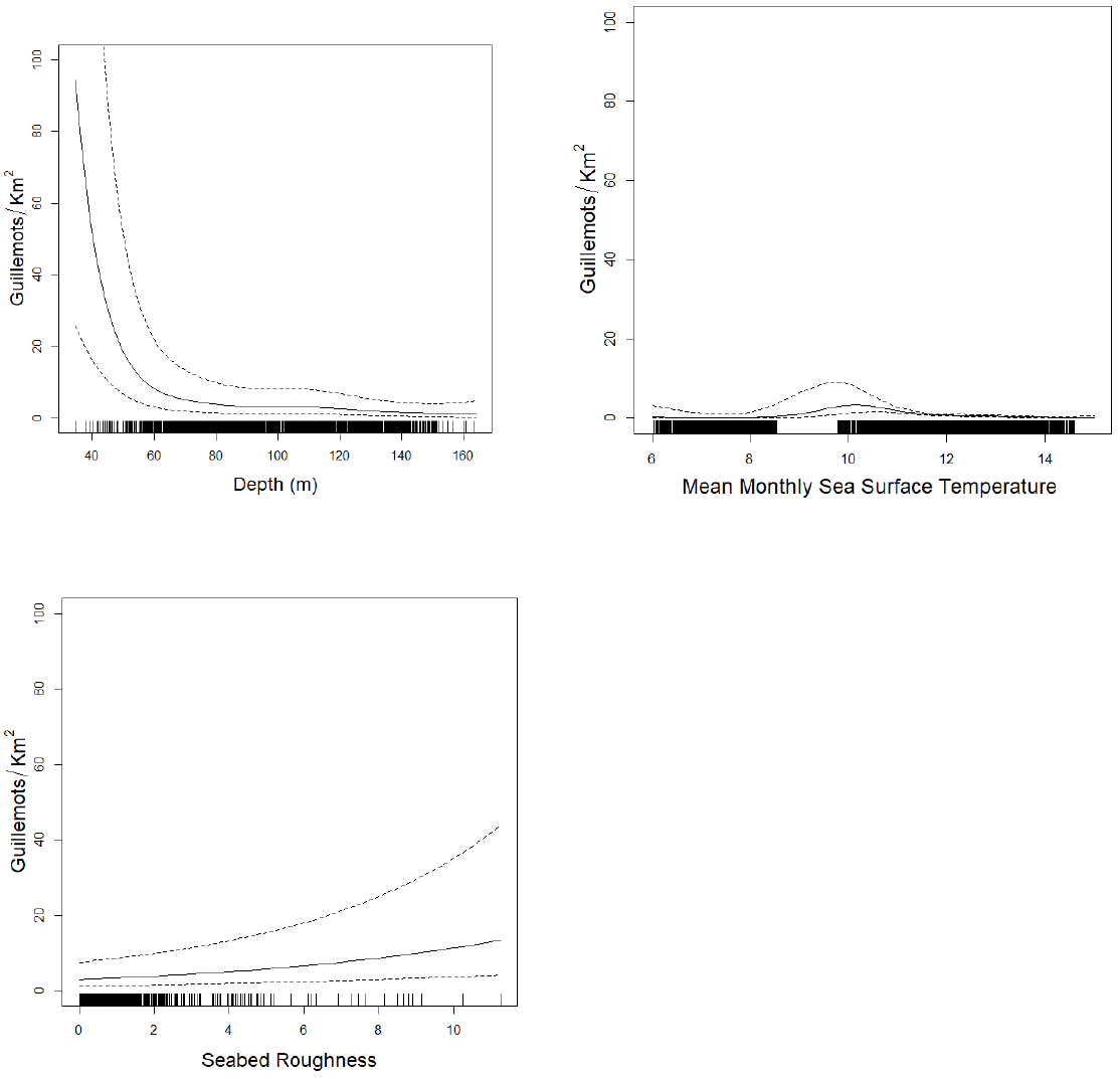
The effects of the non-location variables are given in Figure 59. Note that these are the effects of these variables in the model given the other variables, so they may be very different from the actual marginal effect in the absence of the other variables. This is especially the case for SST which is correlated with Dayofyear (not shown).
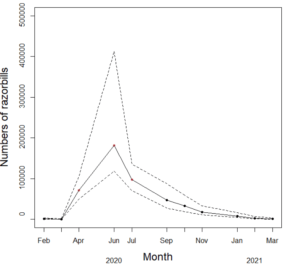
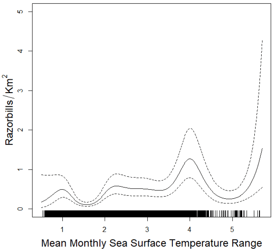
6.3.10 Razorbill
The separate fitted models for breeding and non-breeding season are given in Table 8. The estimated numbers of razorbills in the survey region is given in Figure 60. It shows a strong peak during the breeding season between April and July.
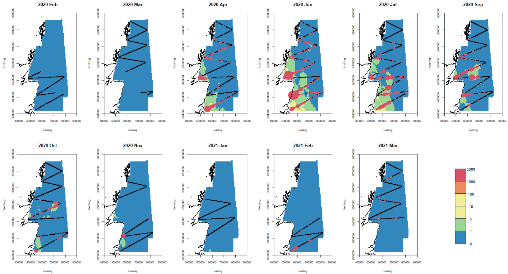
Point estimates of razorbill density for the sampling months along with the confidence bounds are given in Figure 61, Figure 62, and Figure 63. They indicate greatest densities nearer the coast around the Moray Firth, east Grampian region and Firth of Forth, between April and July. There appears to be a hotspot of higher density offshore east of the Moray Firth in late summer and autumn, particularly September and October. The CVs are shown in Figure 64 and are larger in the non-breeding than breeding season. The mean point estimates for breeding and non-breeding season in shown in Figure 65 and shows higher densities in the breeding season at the south western part of the study site.
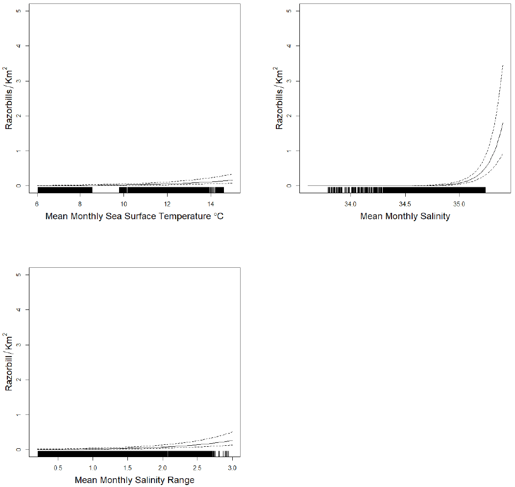
The effect of monthly mean sea surface temperature (SST) in the breeding season model is given in Figure 66, but note that there may be some overfitting of the model here. The effect of SST, salinity and salinity range in the non-breeding season model, is given in Figure 67. They show little obvious relationships although densities are possibly higher at greater sea surface temperatures and salinities. Note that these are the effects of these variables given the presence of location in the model, so may be very different from the actual biological effect.
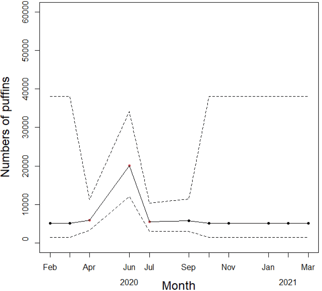
6.3.11 Atlantic Puffin
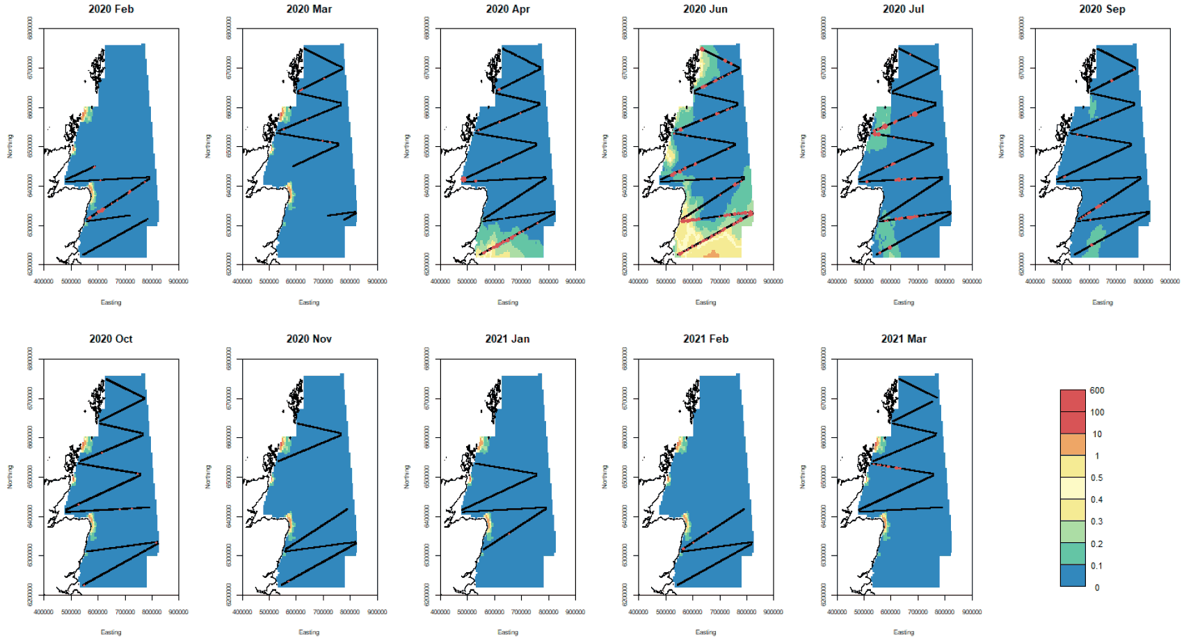
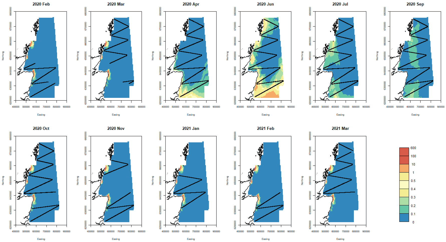
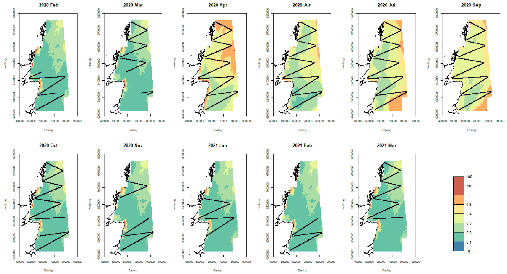
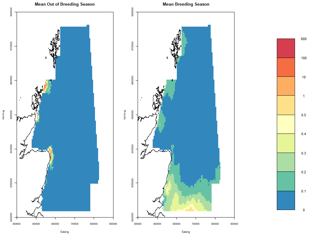
The separate fitted models for breading and non-breeding season are given in Table 8. Estimated numbers through the study period are given in Figure 68. They show a peak during the breeding season between April and July. Point estimates of puffin density for the sampling months along with the confidence bounds are given in the Figure 69, Figure 70 and Figure 71, For this species there were predicted areas of high density near the coast in regions with little survey effort. The CVs are shown in Figure 72 and are higher in breeding than non-breeding season. The mean point estimates for breeding and non-breeding season in shown in Figure 73 and indicate higher densities in the south-western part of the study area during the breeding season.
Greatest densities occurred between April and June particularly in the southern part of the study area, around the Firths of Forth and Tay and east Grampian coast, although high densities are predicted east of Caithness and the Northern Isles where survey effort was low.
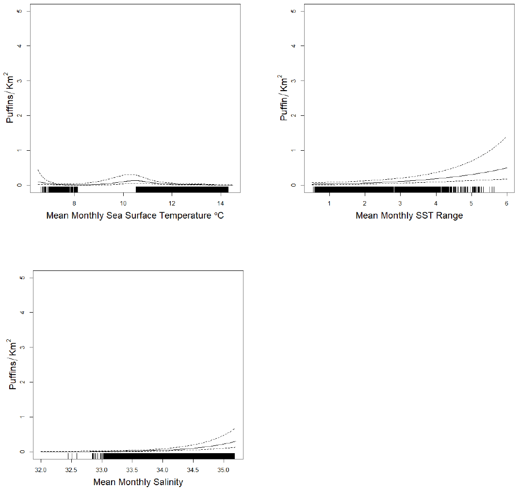
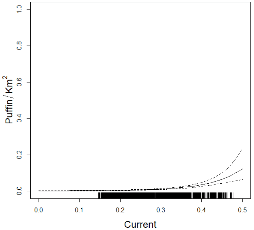
The effect of the non-location variables in the breeding season model is given in Figure 74. The effect of current in the non-breeding season model is given in Figure 75. Note that these are the effects of these variables given the presence of location in the model, so may be very different from the actual biological effect.

6.4 Marine Mammal Species
6.4.1 Minke Whale
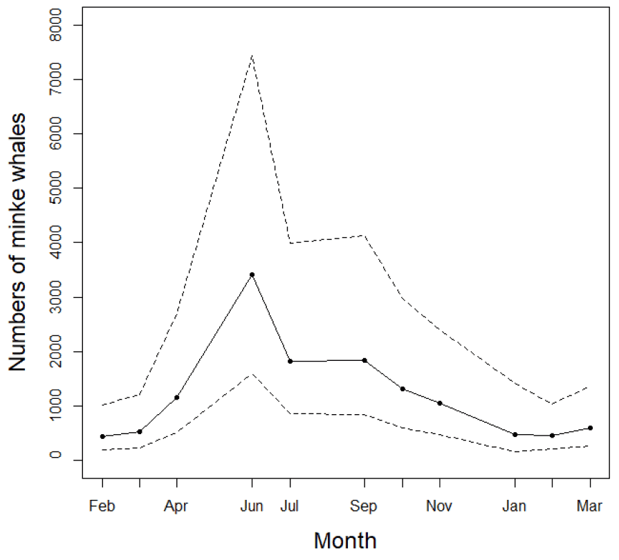
There were only 35 datums out of the 5,036 reduced data set locations with minke whale presences, so a number based spatial model could not be fitted. A binomial presence-absence model was fitted and then numbers were estimated based on the mean number seen per presence. This model is not ideal. Availability was estimated at 0.04. Peak numbers occurred in June followed by a steady decline (Figure 76 Table 9).
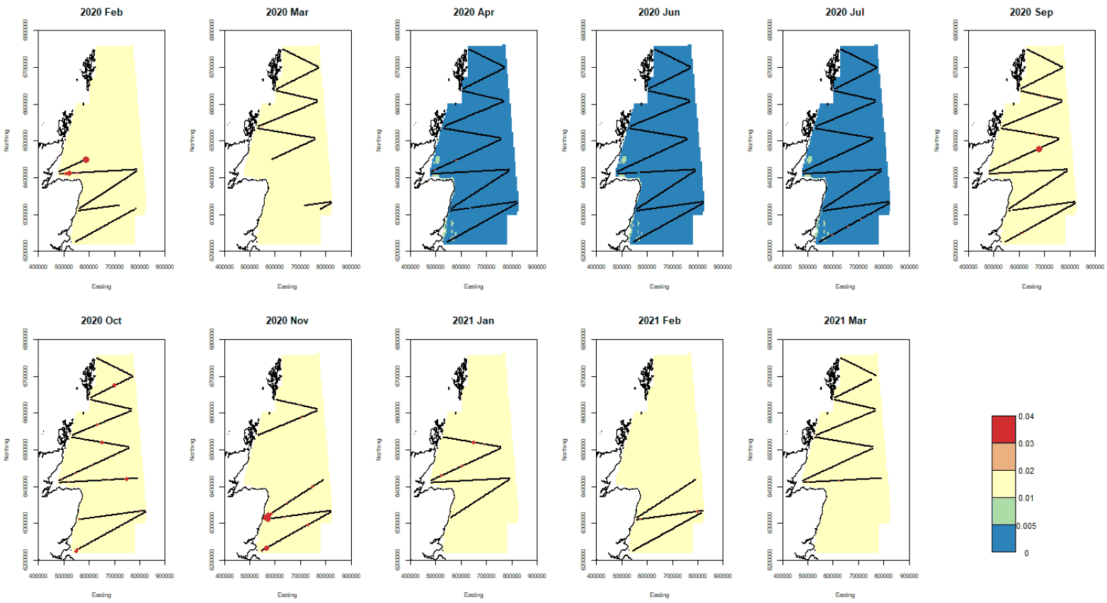
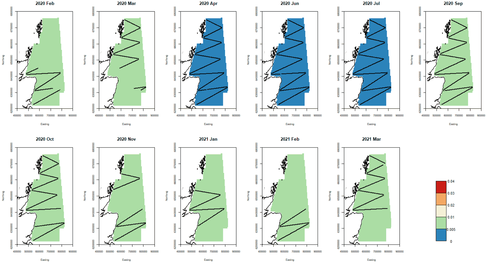
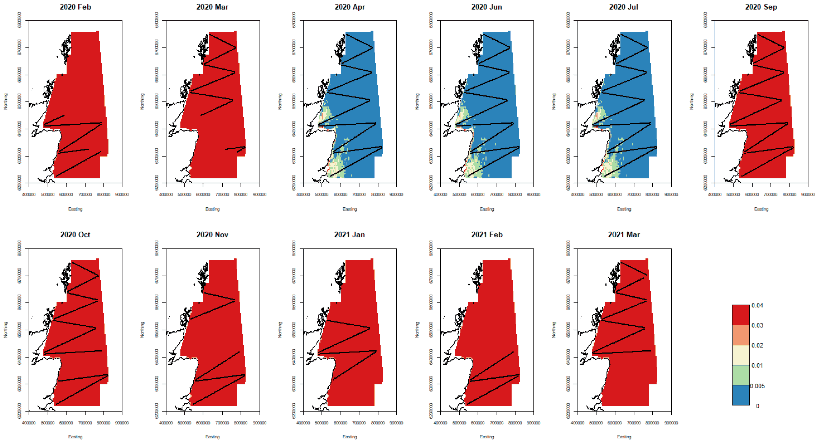
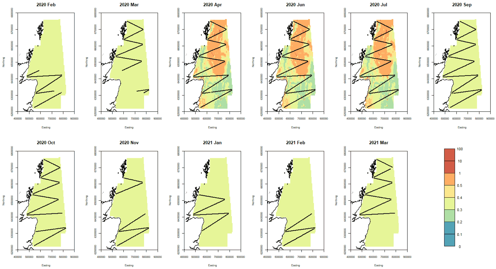
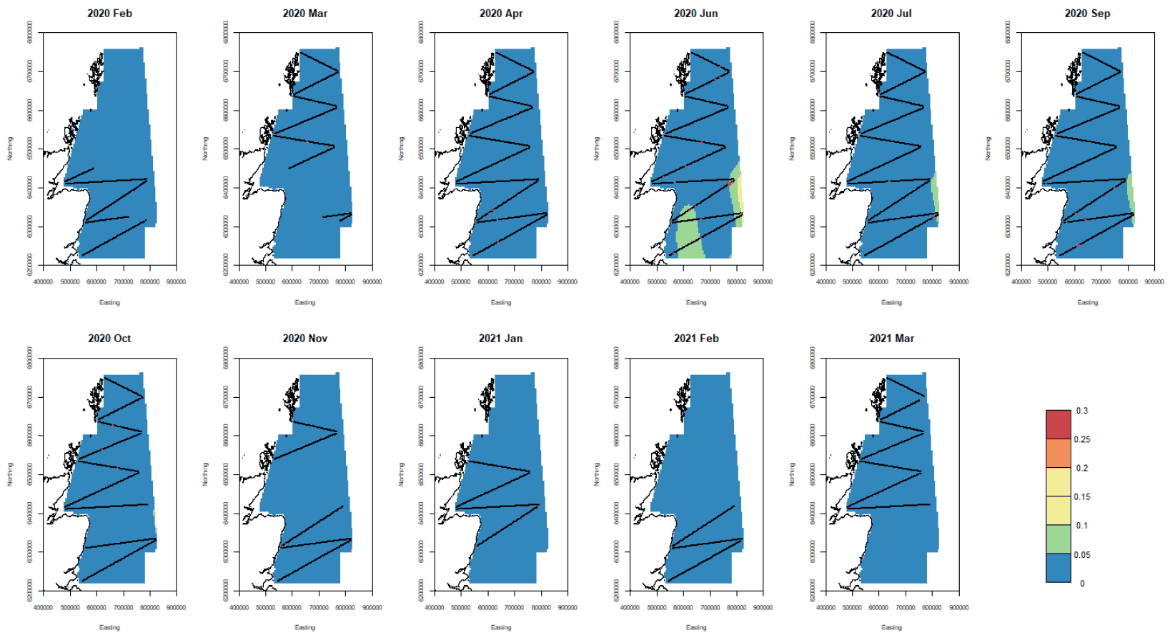
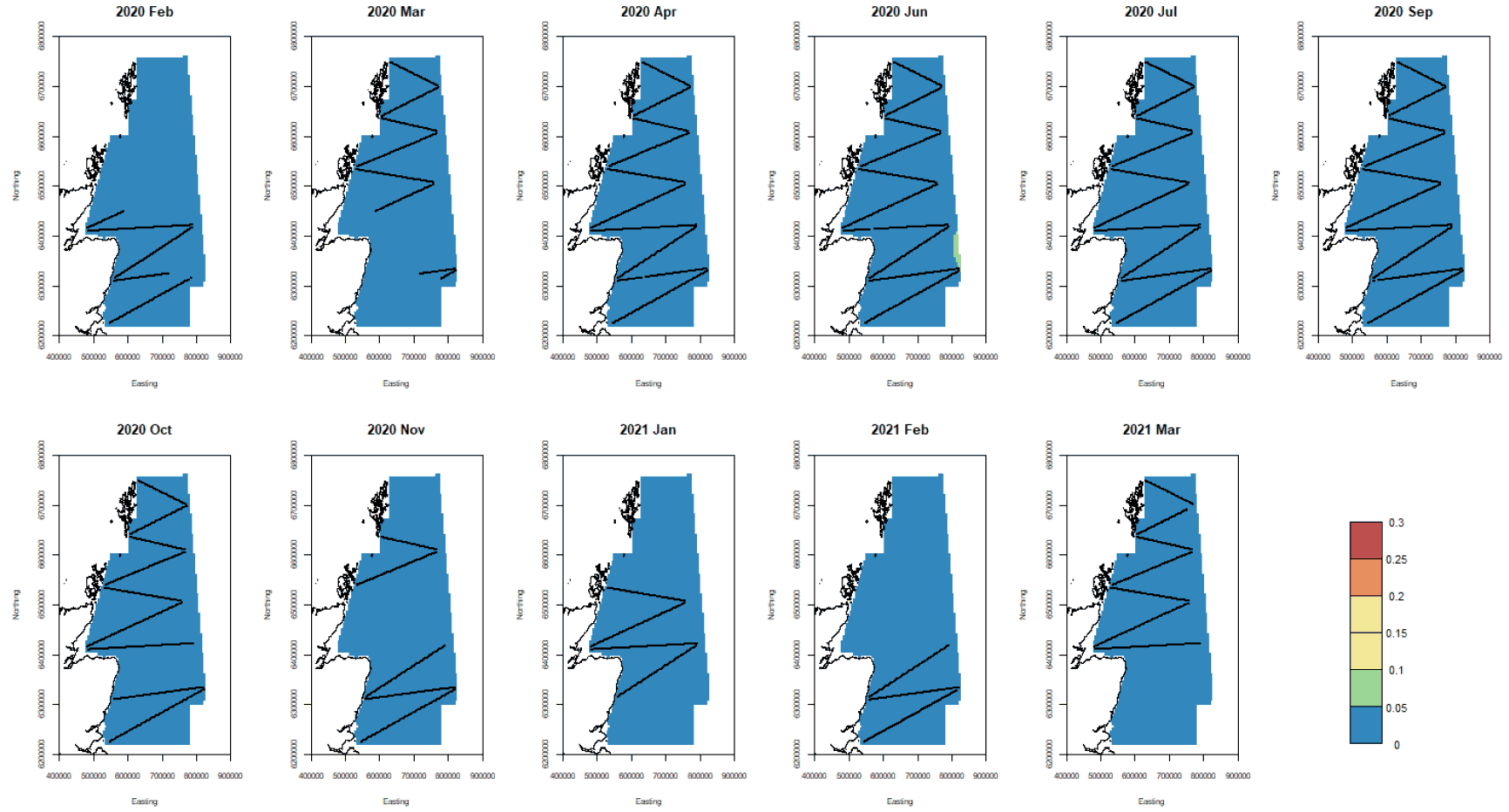
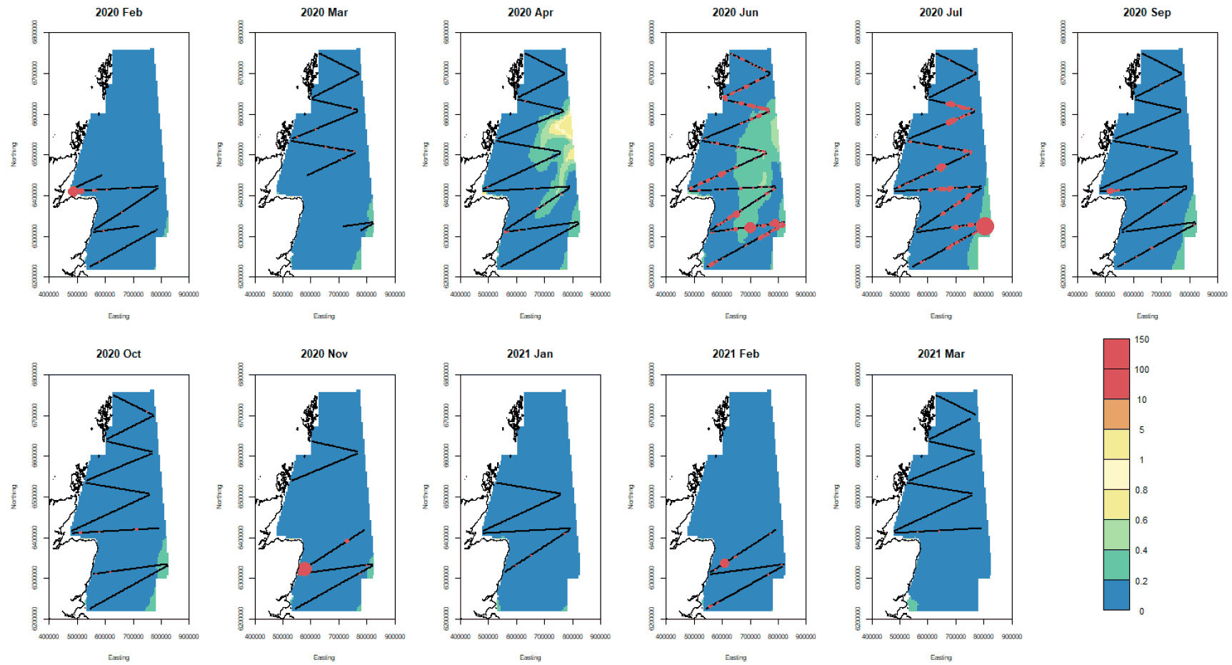
Point estimates of minke whale density for the sampled months along with the confidence bounds are given in Figure 77, Figure 78, and Figure 79. The higher numbers observed in June occurred in two areas: in the north-western North Sea east of the Grampian region and Firth of Forth, and further east in the middle of the North Sea. No CVs were produced for this species.
6.4.2 Common Dolphin
In the case of common dolphins, there were only 18 datums with common dolphin presences. A binomial model of presence was attempted on a reduced dataset from March to July (as no animals were seen outside this time) but no spatial signal could be found (Table 9). The estimates of abundance are therefore 0 outside March to July, otherwise 6170 (95% confidence interval 3530 – 10790), assuming an individual availability at the surface of 0.05.
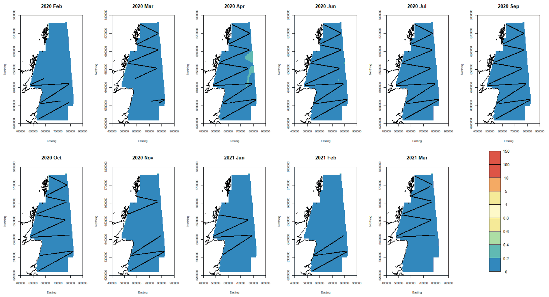
Locations of sightings for common dolphins across the sampled months are given in Figure 80 but no model fits are done. Most sightings occurred in the month of June offshore in the middle of the North Sea although the species was also recorded further north, east of Caithness in March 2020.
6.4.3 White beaked Dolphin
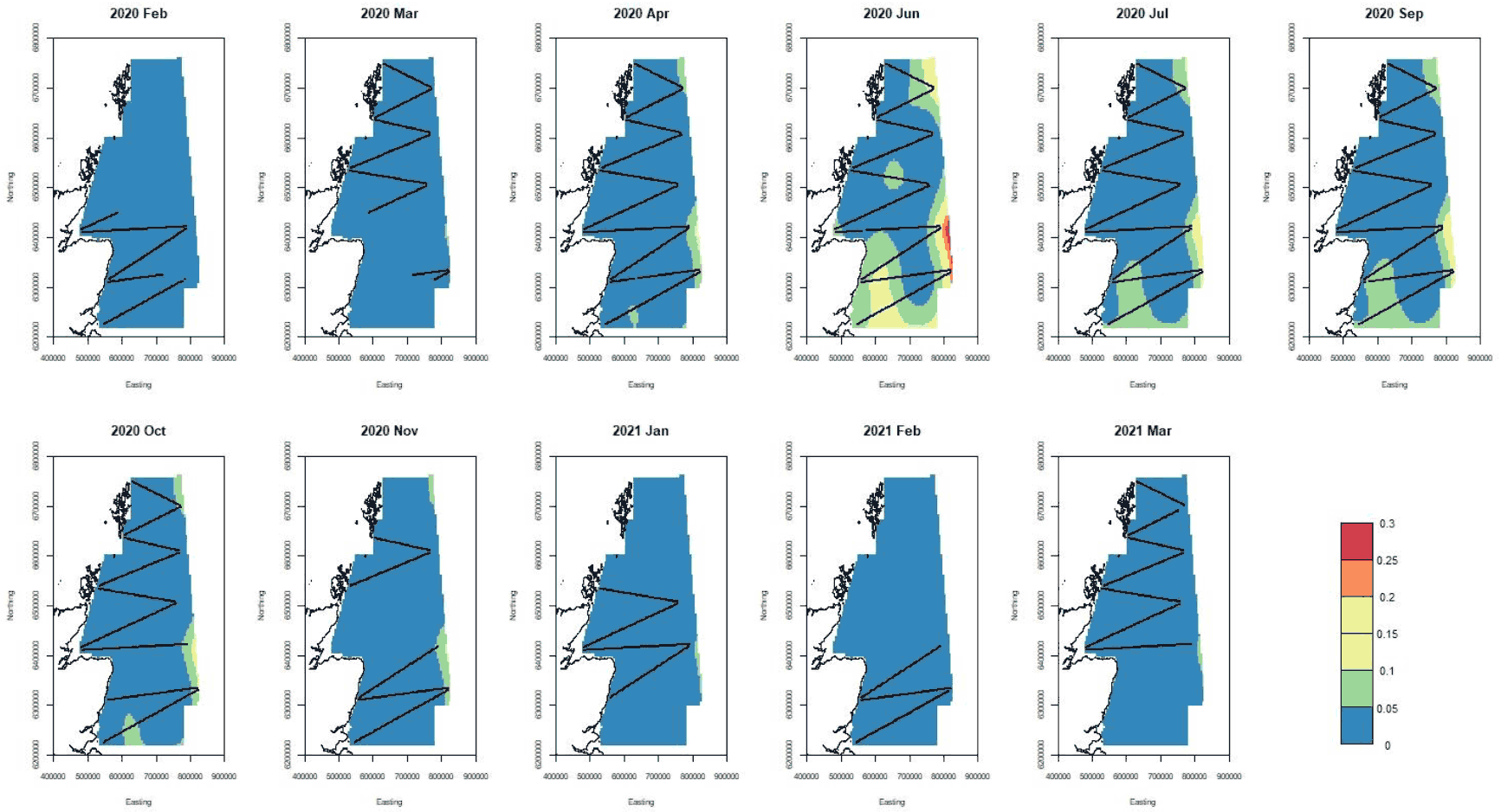
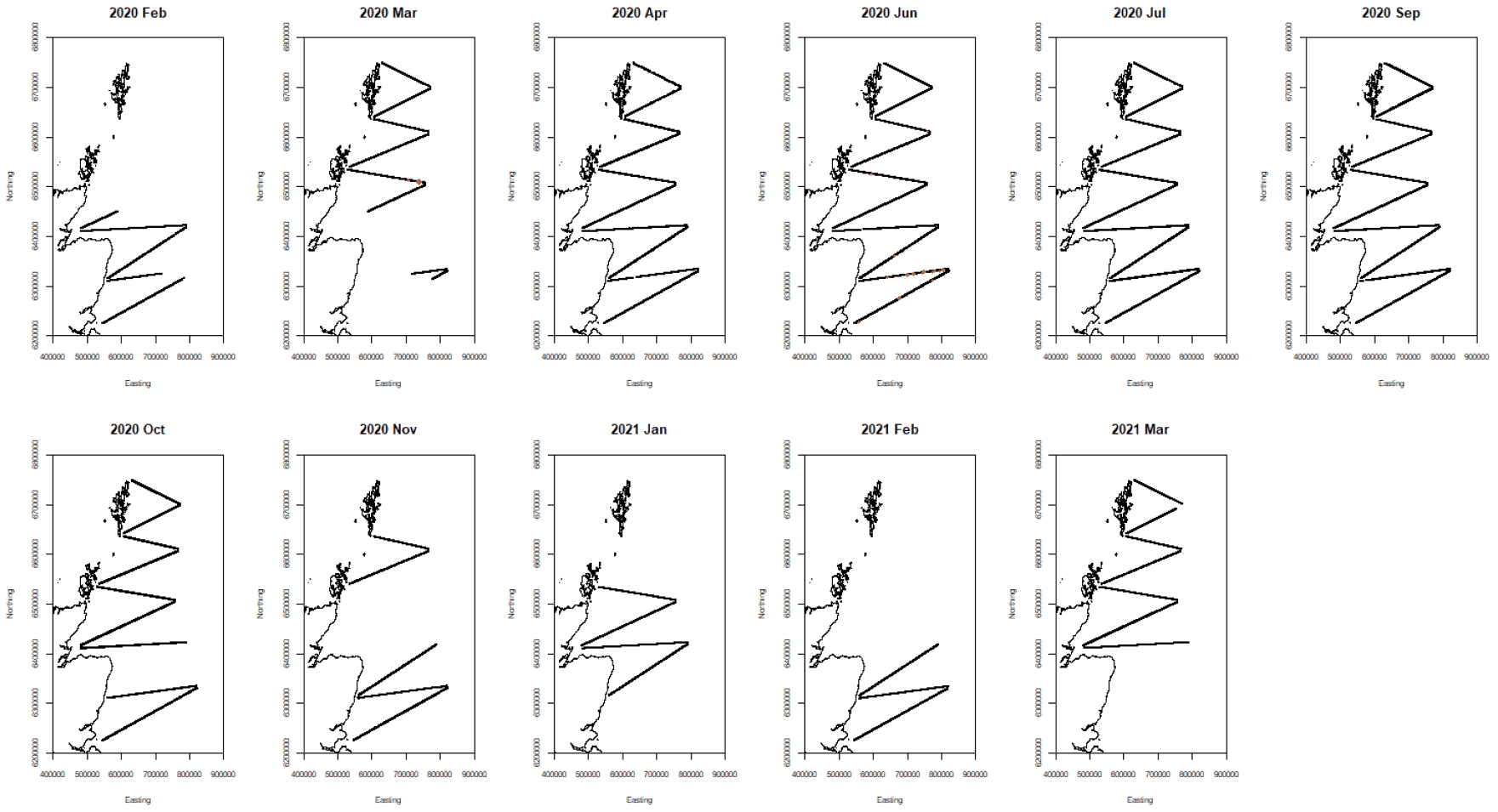
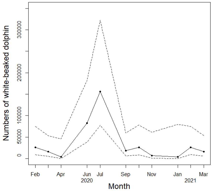
The fitted model of all data is given in Table 9. A model with Dayofyear could not be fitted so instead Month was used as a factor variable. The estimated numbers from the model are given in Figure 81. Although there were sightings in several months of the year, they show a strong seasonal peak in July. Surface availability was assumed to be 0.06.
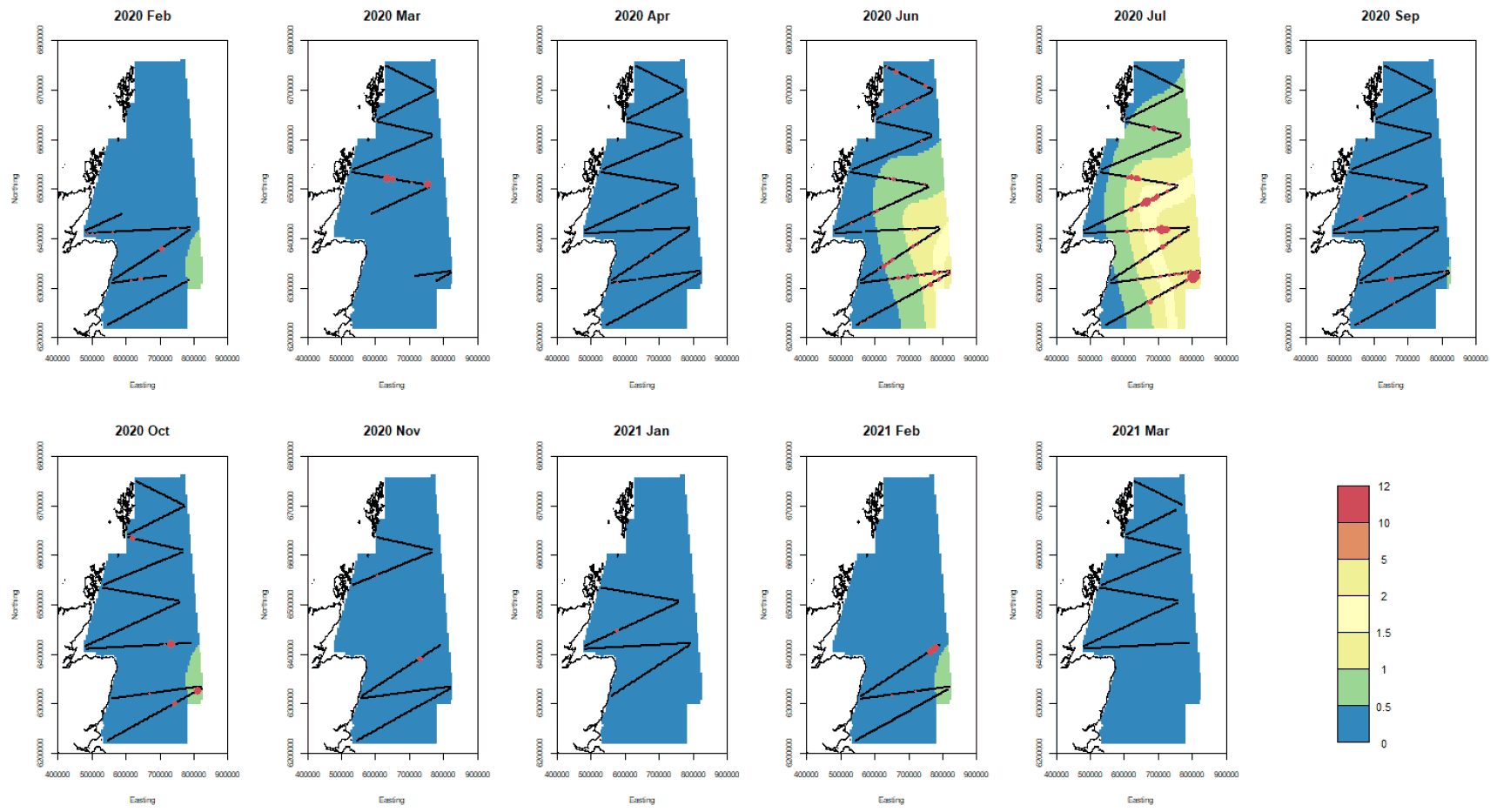
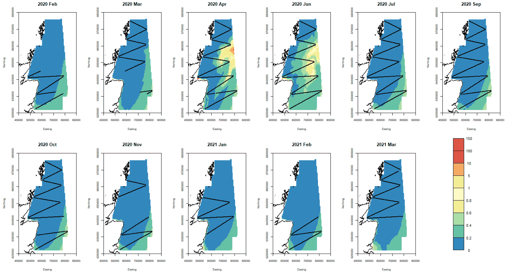
Point estimates of white-beaked dolphin density for the sampled months along with the confidence bounds and CVs are given in Figures Figure 82, Figure 83, Figure 84, and Figure 85. The models indicate a general distribution across the North Sea with highest densities further offshore.
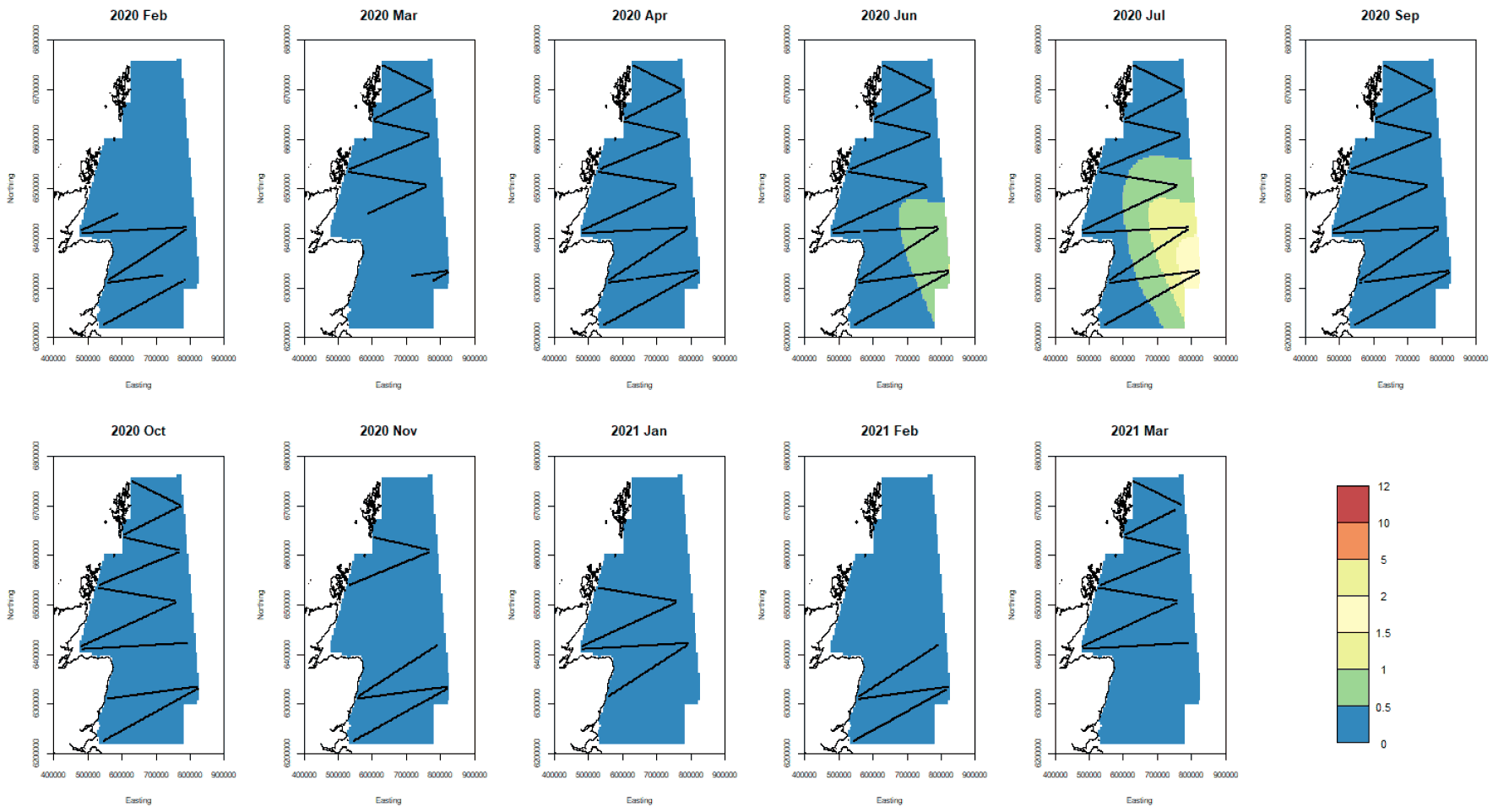
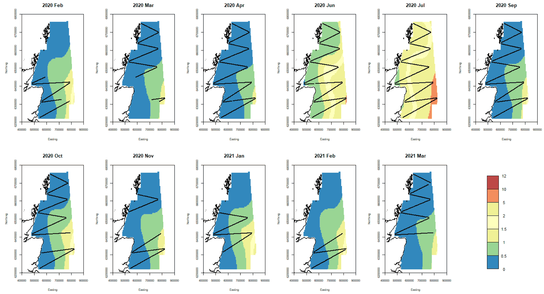
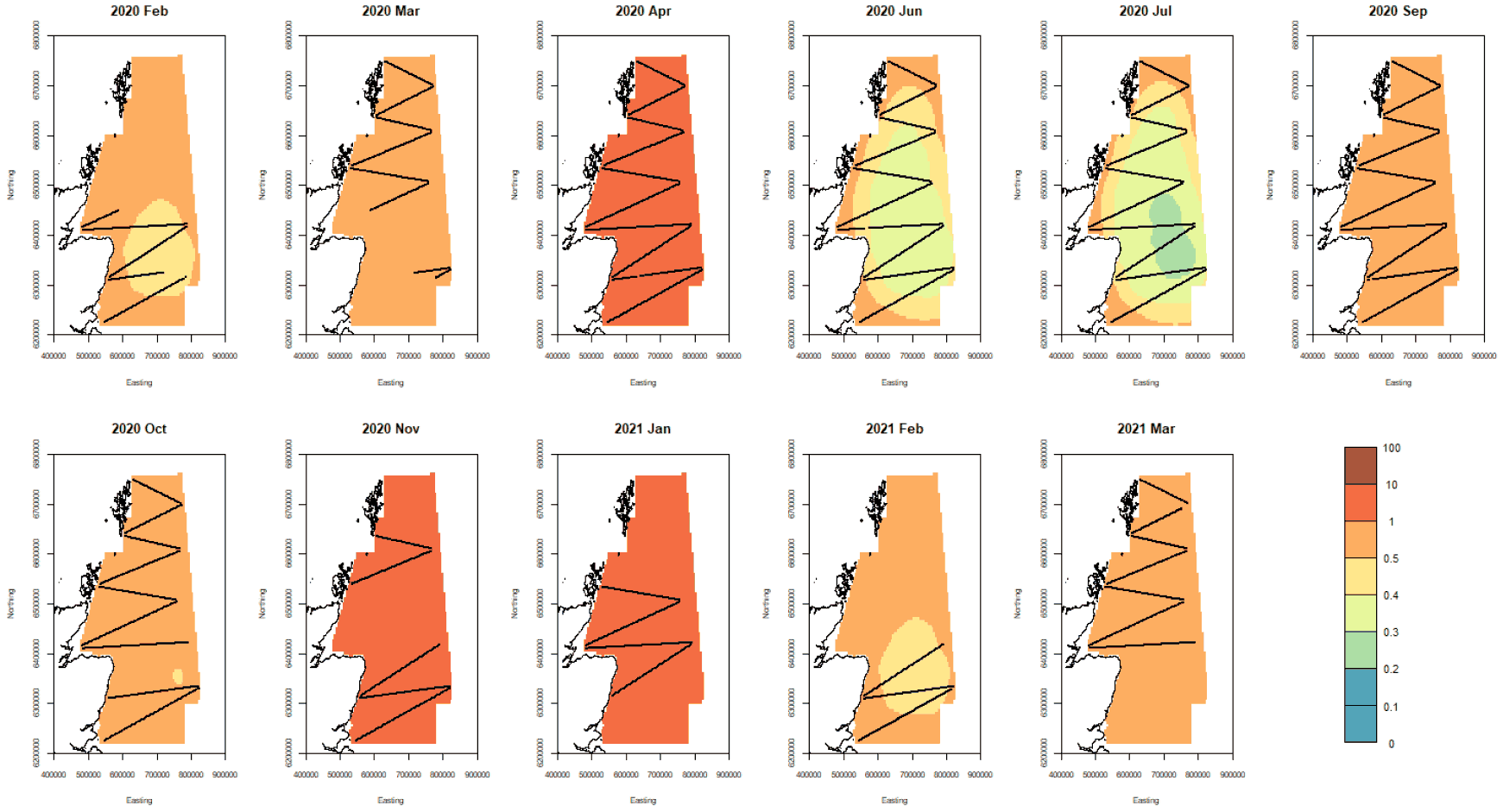
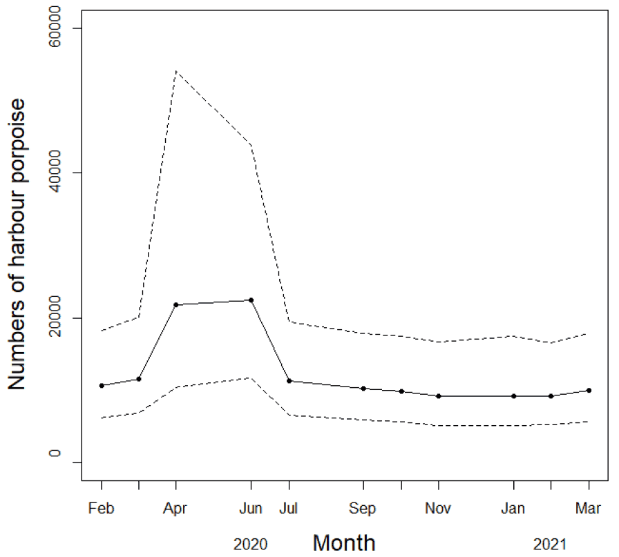
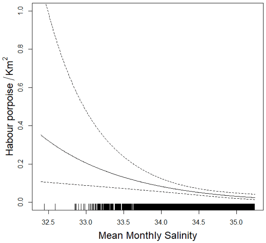
6.4.4 Harbour Porpoise
No model with a correlated error structure could be fitted to the n= 97090 data so the data were further amalgamated into 3-min chunks. This gave a total of 5093 datums. The model is given in Table 9. The predicted numbers over the period of the survey are given in Figure 86. These show broadly similar abundances through the year but with a peak between April and June.
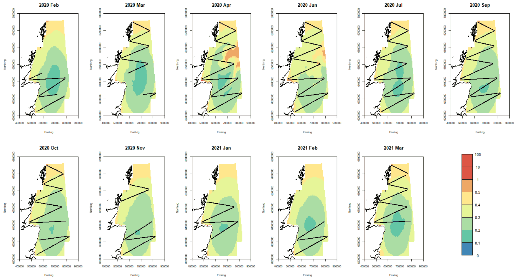
The spatial density surfaces for the sampled months are given in Figure 87, and Figure 89 along with associated uncertainty. They indicate broad distributions for the species in most months, with highest offshore densities east of the Moray Firth and Grampian region.
The effect of salinity on density is given in Figure 91, suggesting there may be higher density where freshwater has a greater influence.
Contact
Email: REEAadmin@gov.scot