Production of Seabird and Marine Mammal Distribution Models for the East of Scotland
This report describes temporal and spatial patterns of density for seabird and marine mammal species in the eastern waters of Scotland from digital aerial surveys. This is important in order for the Government to make evidence-based decisions regarding the status of these species and management.
5. Methods
5.1 Overview of Methods
Here we present a brief summary of the statistical methods and the general approach undertaken to produce the density surfaces, prior to a more detailed description in the later sections. Note that the primary consideration here was to obtain distribution and abundances from the digital aerial survey data. The data under consideration (see below) consisted of counts of animals from digitally referenced images from the survey. We modelled the numbers based on the number of animals detected in photos of known area (“the count method”; see Hedley 2000, Hedley & Buckland 2004, Hedley et al. 2004).
The first stage of the analysis consisted of correcting the observed numbers seen for imperfect identification. The second stage of the analysis involved modelling the resultant estimated densities as a function of space, time and other explanatory variables. The predictions were made from the models over the survey region (see Figure 1). In the case of marine mammals, the resulting predictions were then corrected for surface availability. Thus, monthly indices of abundance could be obtained. Associated with both of the processes is the estimation of the relevant uncertainty. Availability and recognition uncertainty were not incorporated at this stage. All analysis was undertaken in R (R Core Team. 2013).
5.2 Overview of the Data Collection Procedure
The data were collected in the form of temporally and spatially indexed photos from planes collected between February 2020 and March 2021 by APEM Ltd (Figure 1).
APEM’s camera system was fitted into a twin-engine P68 Ravenair aircraft. The plane surveyed at a height of 2,000 feet and a ground speed of 120 knots (138 mph). The aerial digital surveys captured images along ten transects spaced in a saw tooth pattern to achieve full coverage across the targeted area east of Scotland. Data collected approximately two-centimetre ground sample distance (GSD) digital still images. The transect swathe was 960 metres, images were collected continuously (abutting digital still imagery) along the ten transects. The image sea surface area covered was 194 km2, representing 1.5% coverage of the wider surface area. Flights were made in sea states less than 4 on the Beaufort scale.
Typically, several images were taken and processed at the same time. With a total of 242,550 images. However, the counts from simultaneous deployments of the camera were amalgamated if the precise time could be identified to make the data more tractable, creating a dataset of 97,090 location datums each with counts of a variety of species. Figure 1 gives the survey coverage by month.
Survey transects targeted offshore areas beyond 12 nautical miles.
5.3 Predictor Variables
At the spatial modelling stage of the project, animal numbers were modelled considering environmental and biological inputs of potential relevance. Only predictors that can be assigned to all the relevant effort and sightings data were used.
The variables considered are given in Table 2 along with their temporal range. To be of use, the variables must cover the temporal and spatial range of the survey data. Further details are given below.
Variation in depth in the prediction region is shown in Figure 2 and highlights how the majority of the southern part of the study area is at depths of less than 100 metres whereas further north except for the Moray Firth and nearer the coast of east Orkney, depths usually exceeded 100 metres.
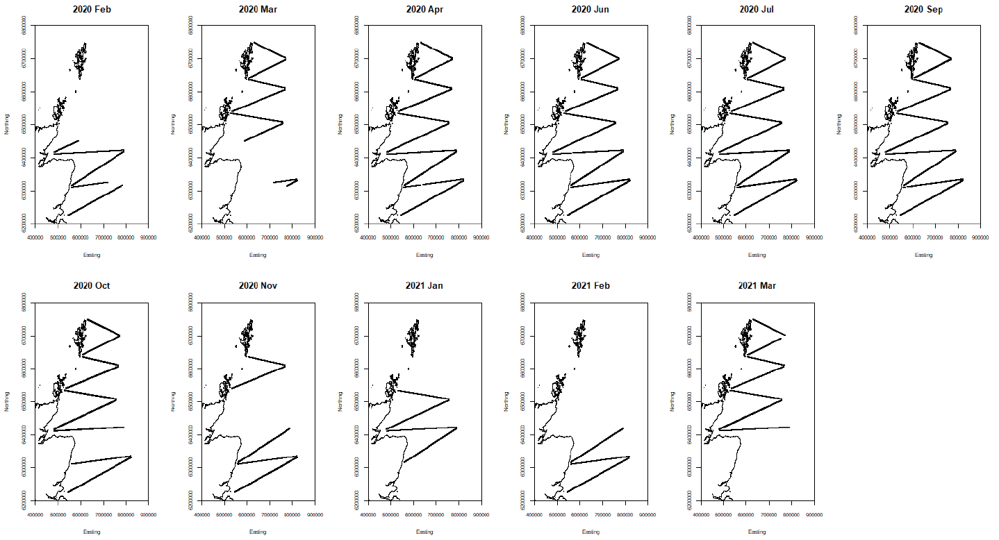
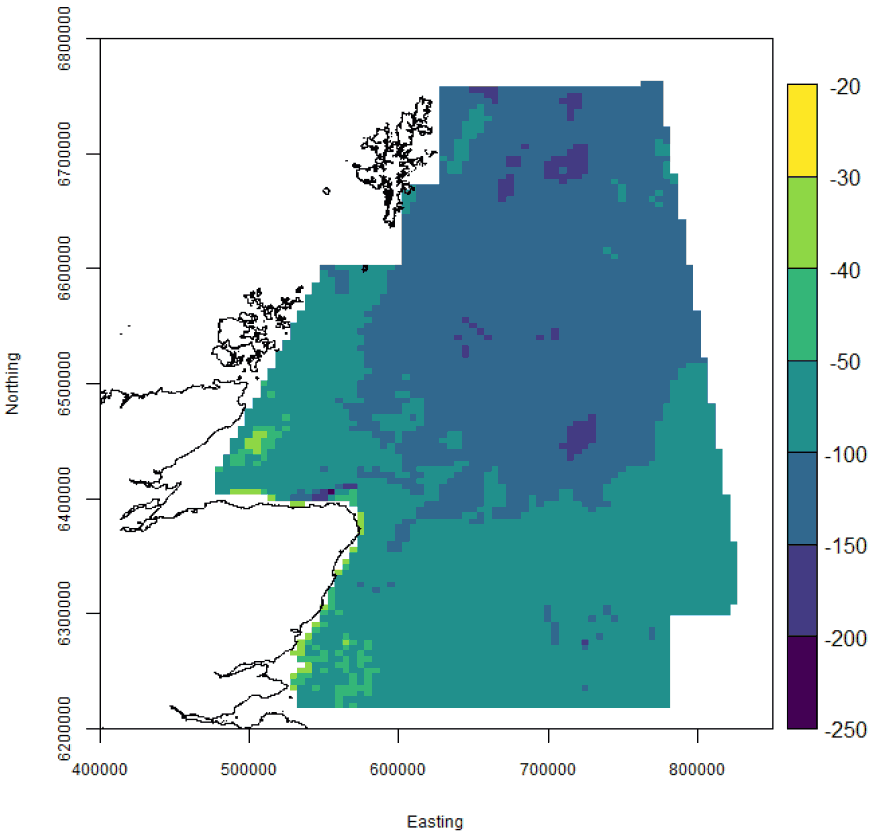
Table 2. Spatial predictors for consideration in modelling.
Position
Description
Easting, Northing assuming UTM30V zone.
Resolution
1 m
Temporal range
Collected on survey
Reference/ link
Position
Predictor
Day of Year
Description
Either from 1st Jan for breeding season only data or from end of breading season for non-breeding season analyses
Reference/ link
Day of Year
Depth
Description
The depth of the seabed. Different depths may support different prey assemblages (i.e., species or age-classes). Benthic prey is also more accessible on shallower seabeds.
Resolution
Available at ~1m but resampled and processed at 1.5km
Temporal range
Static
Reference/ link
EMODNet Bathymetry Portal (https://www.emodnet-bathymetry.eu/)
Monthly Sea Surface Temperature
Description
The mean sea surface temperature (o C) in the calendar month for the survey. Temperature identifies different water-masses, which may support different prey assemblages (i.e species or age-classes).
Resolution
1.5km
Temporal range
Monthly
Reference/ link
From AMM15 FOAM Models, available at the Copernicus Monitoring Service (https://marine.copernicus.eu/)
Seabed roughness
Description
Derived from ‘Depth’ using a terrain ruggedness index (TRI) which represents the mean difference between a focal cell and the 8 surrounding cells. This index identifies areas of rough and uneven seabed including banks, troughs, and complex coastal topography. Such features may promote hydrodynamic features that increase primary productivity and/or aggregate prey (see Cox et al 2018)
Resolution
Available at ~1m but resampled and processed at 1.5km.
Temporal range
Static
Reference/ link
EMODNet Bathymetry Portal (https://www.emodnet-bathymetry.eu/)
Simpson Hudson Stratification Index
Description
Derived from ‘Depth’ and ‘Mean Surface Current Speed’ (log10 (h/u3), whereby h = depth in meters and u = speed in m/s). This index identifies areas likely to remain mixed (<1.9) or become stratified (>1.9) in summer. However, it also describes water column dynamics across the annuals cycle i.e., shallow and turbulent versus deep and non-turbulent. Note that calculations should strictly use depth-averaged current speeds rather than surface current speeds. However, the latter provided comparable measurements, and are sufficient to identify mixed and stratified water in the study area. Prey behaviour may be influenced by water column dynamics, influencing their exploitability. See Scott et al 2010.
Resolution
1.5km
Temporal range
Static
Reference/ link
From AMM15 FOAM Models, available at the Copernicus Monitoring Service (https://marine.copernicus.eu/) and EMODNet Bathymetry Portal (https://www.emodnet-bathymetry.eu/).
Monthly Mean Sea Surface Temperature Range
Description
The range of sea surface temperature (o C) in the calendar month of the survey. High values identify regions of freshwater influence (ROFI) associated with higher productivity (See Cox et al 2018).
Temporal range
Monthly
Reference/ link
From AMM15 FOAM Models, available at the Copernicus Monitoring Service (https://marine.copernicus.eu/)
Monthly Mean Salinity
Description
The mean sea surface salinity (ppt) in the calendar month of the survey. Low values identify mouths of estuaries associated with migratory routes of some prey (See Cox et al 2018).
Temporal range
Monthly
Reference/ link
From AMM15 FOAM Models, available at the Copernicus Monitoring Service (https://marine.copernicus.eu/)
Monthly Mean Salinity Range
Description
The range of sea surface salinities (ppt) in the calendar month of the survey. High values identify mouths of estuaries associated with migratory routes of some prey (See Cox et al 2018).
Temporal range
Monthly
Reference/ link
From AMM15 FOAM Models, available at the Copernicus Monitoring Service (https://marine.copernicus.eu/)
Mean Surface Current Speed
Description
The mean sea surface current speeds (m/s) across a typical spring-neap cycle. Areas of high current speeds generally contain hydrodynamic features suspected to aggregate prey items and/or increase encounters with prey (See Benjamins et al 2015).
Temporal range
Static
Reference/ link
From AMM15 FOAM Models, available at the Copernicus Monitoring Service (https://marine.copernicus.eu/)
Colony indices for each seabird species
Description
Colony Index is an index (0-1) representing the distance to colonies weighted by the relative size of that colony.
It assumes an exponential decay in animal densities with distance from colony, linked to a homogeneous dispersal across all directions.
Temporal range
Static
5.4 Adjustments for Non-recognition
Some individual animals were not identified to species in the photo survey although they were identified to family (birds) and order (marine mammals). Such individuals were allocated to species as follows by using, where possible, species ratios obtained from the MERP database (see Waggitt et al. 2020). The MERP database included vessel, visual aerial and digital aerial data collected across the region by a much larger set of data providers and spanning a much longer time period (1980-2018). Vessel surveys in particular are better at identifying animals to species (Johnston et al. 2015, Waggitt et al. 2020). Ratios of abundance between similar species (e.g. razorbill and guillemot) have not changed very much over those years (Stone et al. 1995, Mitchell et al. 2004, JNCC 2016, Potiek et al. 2019, Waggitt et al. 2020), and so this was considered a valid procedure.
For each locality with an unidentified animal, all observations within 50 km of the locality were extracted from the MERP database. The ratio of species in the relevant group (e.g. skuas, auks, “dolphins”, “dolphin or porpoise” etc.) was used to allocate the vaguely identified images to species for that location.
5.5 Density Surface Modelling
Model selection proceeded as follows. The data were counts and contained large numbers of zeros, therefore the response data were likely to be more variable (i.e. overdispersed) than assumed under some distributions. This variability needed to be accommodated under the selected model. Furthermore, the observations were close together in space/time and these observations were likely to be more similar than observations distant in space/time. Covariate data can potentially explain part of the correlation in the counts; however, it is unlikely that the correlation will be explained in full. In the case of marine mammals, the data were initially considered as a complete set. Backwards model selection initially proceeded assuming the datums were independent. Model selection was by automatic smoothing with mgcv (Wood 2017) using restricted maximum likelihood (REML). Then, after the model was reduced, the residuals were tested for autocorrelation (by examination of partial and full autocorrelation plots of the residuals) to identify the interval at which datums became independent. Further variables were then removed on a wholly independent reduced data set after several models were fitted with different subsets of data (i.e. different reduced datasets were created by taking the nth datapoints from different start points). Finally, the full dataset (n = 97,090) was fitted using the reduced variable set within a mixed-model GAM (GAMM, Wood 2017) with an appropriate correlation error structure. More model reduction was allowed. The use of GAMMs allowed smoothed responses to be fitted to the predictors. Family error structure in this high zero frequency data set was considered to follow a negative binomial or Tweedie distribution. Diagnostic plots were examined to evaluate the best model.
If the model had a negative binomial error structure, it typically had the following form:
yi =exp(β0 + s(Eastingj, Northingi)+s(X1i) + s(X2i) + εi
where s(Eastingj, Northingi) is the 2D smooth of Easting and Northing for the ith point and X1 and X2 represent smooths of single predictors (see below for details) of which thre could be a large number (see below).
In the case of birds, the data were first split into breeding and non-breeding season (see Table 3) and then analysed as above for each season (although the candidate variable set was different, see Table 7).
Table 3. Bird seasons used in this analysis (following Searle et al. 2022).
Northern fulmar
Breeding season
April - August
Non -breading season
September - March
Northern gannet
Breeding season
April - October
Non -breading season
November - March
Great skua
Breeding season
April - July
Non -breading season
August - March
Common gull
Breeding season
April - July
Non -breading season
August - March
Species
Lesser black-backed gull
Breeding season
April - July
Non -breading season
August – March
Herring gull
Breeding season
April - July
Non -breading season
August – March
Great black-backed gull
Breeding season
April - July
Non -breading season
August - March
Black-legged kittiwake
Breeding season
April - August
Non -breading season
September - March
Common guillemot
Breeding season
April - July
Non -breading season
August - March
Razorbill
Breeding season
April - July
Non -breading season
August - March
Atlantic puffin
Breeding season
April - August
Non -breading season
September - March
For some species, model fitting on the reduced dataset (n = 97,090) proved impossible, so the data were further reduced to 5,093 by binning the data into 3 min bins (based on the number of photos taken). This reduced but did not eliminate the autocorrelation but made modelling more tractable. In the case of bird species, a Season factor variable was added to the models to allow different relationships across seasons in these models that considered all the data at the same time.
5.5.1.1 Predictions
Predictions from the models were made on a 5 km by 5 km resolution easting and northing grid with confidence intervals directly calculated from the estimated cell standard errors. The results were then corrected for availability (see below).
5.5.1.2 Availability adjustments
The proportion of animals available at the surface has to be considered. For marine mammals, an index of availability at the surface for each sighting was made by considering the reported proportion of time the animals spend at the surface. The probability of a mammal being available at the surface was given by
Proportion(Avail)=(E[s])/((E[s]+E[d]))
where s = surface time, d = dive time. The process in the context of this survey is instantaneous so no correction for observation time is necessary. No correction for availability was made for seabirds. The sources for species availability at the surface for diving marine mammals are summarised in Table 4.
Table 4. Mean surface and dive times used for individuals of target species.
Minke whale
Mean surface time (mins)
0.067 (Anderwald 2009) 0.044 (Gunnlaugsson 1989) 0.053 (Joyce et al. 1989 off Svalbard)
Mean dive time (mins)
1.311(Joyce et al. 1989)
White-beaked dolphin
Mean surface time (mins)
0.058 (P.G.H. Evans, unpublished data)
Mean dive time (mins)
0.917 (M. Rasmussen pers. comm.)
Species
Common dolphin
Mean surface time (mins)
0.058 (P.G.H. Evans, unpublished data)
Mean dive time (mins)
1.0 (Lockyer & Morris 1986, Lockyer & Morris 1987, Mate et al. 1995)
Harbour porpoise
Overall availability in 0 – 2m band 0.615 from Teilman et al. 2013
Contact
Email: REEAadmin@gov.scot