National Electrofishing Programme for Scotland (NEPS) 2021: analysis

Results

Meteorological and hydrological context

There was considerable regional variability in rainfall during summer 2021 (Fig. 5). In July and to a lesser extent August, average or above average rainfall was seen in the east, while the west and north experienced unusually dry conditions. In September the west and south-east experienced lower than average rainfall, while the rest of country was characterised by near average conditions. In October much of Scotland experienced above average rainfall, with the greatest volumes falling in the south and west in particular. These patterns of spatio-temporal variability in rainfall resulted in very lows flows across the west in July, with more average conditions in August and September (Fig. 6). Flows were around or above average on most rivers in October, with particularly high flows in the south west.

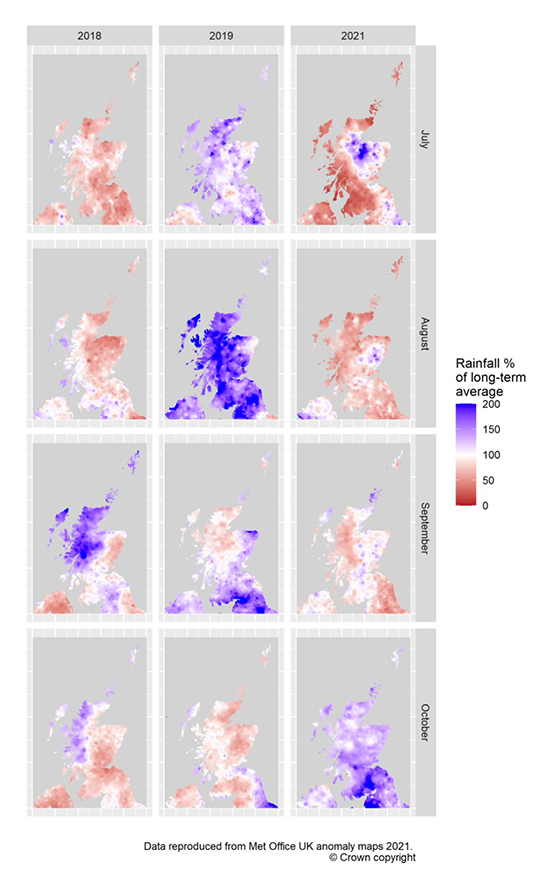
Figure 5 Percentage of long-term average rainfall for July-October when electrofishing was undertaken. Reproduced from MET Office (2021) UK actual and anomaly maps.

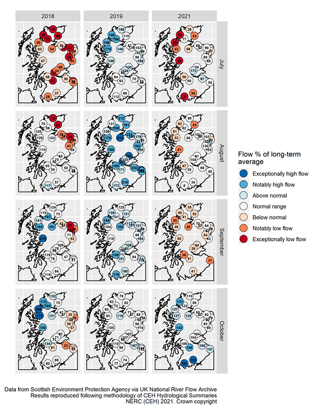
Figure 6 River flows across Scotland during the electrofishing season compared to a 20-year baseline (1981-2010). Colours indicate the 2018, 2019 and 2021 flow ranking relative to baseline years.

Capture Probability (P)

The final capture probability model for salmon and trout was:

logit P ~ Species + Lifestage + Pass + Lifestage:Pass + Organisation-Team + Year + Altitude + Species:Altitude + s(UCA) + s(Gradient) + s(DoY:Lifestage) + s(HA)

where s() denotes smoothed responses and : indicates an interaction term (Fig. 7).

Capture probability was higher for trout than salmon (Fig. 7A), for parr than fry and the first pass versus subsequent passes (Fig. 7B). The reduction in capture probability between the first and subsequent passes was also greater for parr than fry. Capture probability varied temporally with Year (Fig. 7C) and DoY (Fig. 7E). Year was a positive linear effect. DoY was a modal response varying by lifestage where modality was greater for fry than parr, the latter exhibiting a more linear positive response.

Capture probability varied spatially with Altitude, Gradient, UCA and HA. The response was negative with Altitude (Fig. 7F), Gradient (Fig. 7G) and UCA (Fig. 7H). The response to Altitude also varied between species, with stronger negative effects for trout than salmon. There were complex spatially correlated regional patterns in capture probability associated with HA (Fig. 7I).

Capture probability varied substantially between Organisation - Teams (Fig. 7D), although major differences were typically between Organisation, rather than between Teams within Organisation over time (not shown). Few Organisations routinely work outside their local area of responsibility. This limits contrast in the dataset and makes it challenging to separate regional (HA) and Organisation effects (Organisation - Team). To address this issue Figure 8 combines the effects of Organisation and HA for those Organisation - Teams undertaking sampling for NEPS 2021.

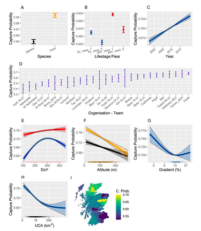
Figure 7 The effects of species (A) Lifestage : Pass (B), Year (C), Organisation - Team (D) Day of the Year : Lifestage (E), Altitude : Species (F) Gradient (G) Upstream Catchment Area (H), and Hydrometric Area (I) on capture probability. Where effects differed between Species or Lifestage they are plotted separately for salmon (black), trout (orange), fry (blue), parr (red). All effects are scaled to the mean fitted first pass capture probability. Approximate 95% pointwise confidence intervals are shown as shaded areas or vertical lines. A rug indicates the distribution of the data on the x-axis. Only Organisation Teams contributing to NEPS in 2021 are shown.

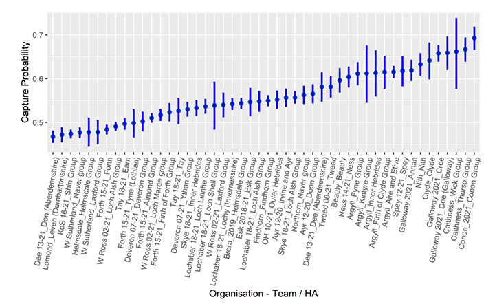
Figure 8 Combined partial effect of Organisation - Team and HA on capture probability. All effects are scaled to the mean fitted first pass capture probability. Approximate 95% pointwise confidence intervals are shown as vertical lines. Only Organisation - Teams contributing to NEPS in 2021 are shown.

Site-wise estimates of abundance (salmon and trout) and status (salmon): NEPS 2021

Estimates of the density of trout and salmon from NEPS 2021 are shown in Figures 9 and 10 respectively. Higher trout fry densities were observed at sites in the Tweed and the north-east, with generally lower densities in the north and west. Trout parr densities appeared less spatially variable with relatively high densities in the north and north-west.

Many NEPS 2021 sites contained no salmon fry (black points, Fig. 10A) and / or parr (Fig. 10B) although patterns of spatial variability were less clear than in previous years. Lower densities of fry were typically observed in the central belt, west coast mainland and the north-east corner. Salmon parr densities were generally higher in northern and eastern areas.

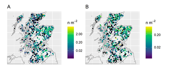
Figure 9. Maps showing spatial variability in trout densities for fry (A) and parr (B). Black points indicate sites where no fish (of the relevant life-stage) were caught.

Not all rivers are expected to produce the same number of juveniles due to spatial variability in habitat quality and thus carrying capacity. In the case of salmon, this is captured by spatial variability in the benchmark (Malcolm et al., 2018, Fig. 2). Unfortunately, a benchmark is not currently available for trout. Thus, only the performance of salmon at individual sites can be assessed through comparison with the benchmark (Fig. 10 C, D). NEPS 2021 data showed a wide range of performance against the benchmark, but sites where observed densities were below the benchmark dominated the picture. The only exceptions to this general pattern were the rivers on the east coast of Scotland, north of the Moray Firth and in the Outer Hebrides, although areas in the south-west around the Solway coast also appeared to perform well, at least in terms of fry.

While the percentage difference plots (Fig. 10 C, D) provide a useful indication of the status of sites, they do not differentiate between poorly performing unproductive sites and poorly performing productive ones. From a fisheries management perspective, the latter is arguably of more concern and is illustrated in Figure 10 (E, F). Production is often substantially below expectation across much of the country, although the effect appears less severe in the north. The underperformance of some sites in the Ness appears particularly marked, reflecting low observed densities and changes in the sample frame to include larger 5^th order rivers where benchmark densities are higher (Fig. 2).

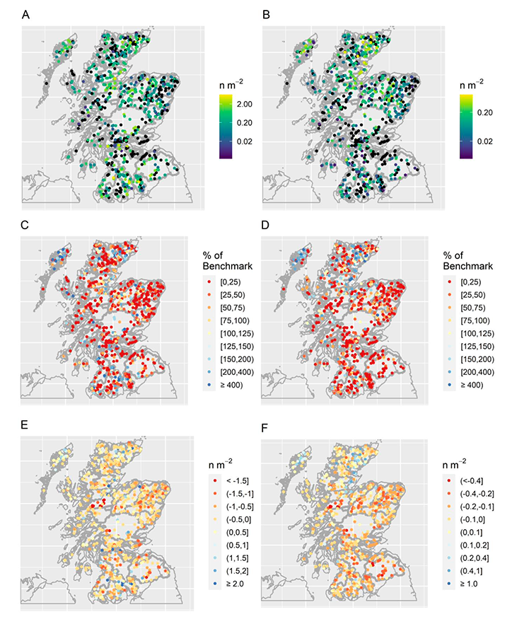
Figure 10. Maps showing spatial variability in observed salmon densities (A, B) together with their percentage (C, D), and absolute (E, F) performance against benchmark. Panels A, C and E show the results for fry. Panels B, D and F show results for parr. Black points (panels A and B) indicate sites where no fish of the relevant life-stage were caught.

National and regional assessments of abundance and status (salmon): NEPS 2021

Changes to the NEPS 2021 survey design both in terms of strata and sample frame (see Methods) made direct comparisons between years impossible without post-stratification and exclusion of some samples (see comparing estimates of abundance between years, below). Regional differences in the characteristics of the sample frames, in particular the inclusion of 5^th order rivers in some regions also reduced comparability of density data between regions. However, spatial variability in the benchmark was able to account for regional variation in the sample frame thereby allowing for valid comparison of NEPS Grades between regions.

At the national scale (excluding rivers above impassable barriers in the Forth) salmon fry densities exceeded the benchmark indicating that fry densities were generally healthy and would achieve a Grade 1 classification (Fig. 11). The situation was starkly different for salmon parr where mean densities were around 60% of their benchmark. Taken together this would result in a Grade 2 classification for the country as a whole.

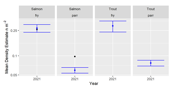
Figure 11 Mean density estimates of salmon and trout, fry and parr for the NEPS 2021 survey. Blue points and error bars indicate mean density estimates and 2-sided 90% confidence intervals. Black points indicate the target benchmark (only available for salmon). Areas above impassable barriers in the Forth region have been removed from the national analysis, although areas above Shin dam have been retained.

Regional (strata level) differences in benchmark densities were greater in NEPS 2021 than in previous years (Figure 12). Higher benchmarks were associated with regional sample frames that were dominated by larger low altitude rivers, at intermediate to high distances to sea (e.g. Conon). In contrast, the presence of many smaller rivers resulted in lower regional benchmark densities (e.g. Lochaber). The effect of removing smaller rivers and adding larger rivers (5^th order rivers) to the sample frame between 2018-19 and 2021 was thus to increase the benchmark density in affected regions. This is most clearly seen in the case of the Ness, where changes to the sample frame resulted in sampling a substantially greater proportion of larger rivers.

By combining regional density estimates, their uncertainty and regional benchmark densities, it was possible to assess spatial variability in the status of salmon (Figures 12 and 13). Salmon fry, which reflected spawner numbers from 2020, were generally characterised by higher grades than salmon parr which reflected spawner numbers from 2019 and earlier years. There were pockets of Grade 1 for salmon fry in the south-west (Annan, Nith, Ayrshire), Firth of Forth, Tay and the north (Beauly, Conon, Helmsdale, Caithness, Northern, Outer Hebrides, Skye and Lochalsh). In the case of salmon parr only regions to the north attained a Grade 1 (Beauly, Conon, Brora, Helmsdale, Caithness, Northern, Outer Hebrides and Wester Ross). Overall grades were also patchy, with Grade 1 regions only observed in the north (Beauly, Conon, Brora, Helmsdale, Caithness, Northern, Outer Hebrides and Skye and Lochalsh) and south-west (Ayrshire). The river Shin (above Shin dam) was the only Grade 3 stratum in the north. This is perhaps unsurprising as Shin dam is a substantial barrier which is classified as impassable by SEPA, primarily for its impacts on downstream migration.

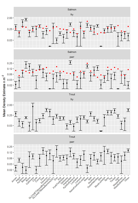
Figure 12 Plots showing density estimates (black points), with associated 2-sided 90% confidence intervals for each of the strata included in NEPS 2021, separated by species and lifestage. In the case of salmon red points indicate the benchmark (expected densities) against which estimated densities can be compared to determine performance grade.

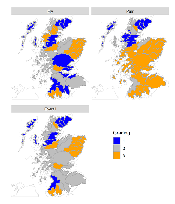
Figure 13. Maps showing NEPS grades for salmon fry, parr and overall grading (fry and parr)

Relationships between Strahler river order and the habitat characteristics of surveyed river reaches

The percentage of riffle and run habitat that was surveyed increased with Strahler river order, while the percentage of surveyed pool habitat declined (Figure 14). This could reflect genuine spatial variability in channel characteristics or increased use of micro-siting on larger rivers to avoid surveying deeper pool habitat.

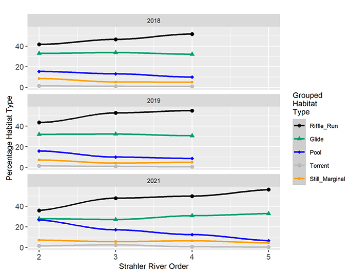
Figure 14 Relationships between Strahler river order and the percentage of different habitats that were surveyed. Rows indicate the different NEPS survey years. Fifth order rivers were only surveyed in some regions in 2021.

Relationships between Strahler river order, mean observed densities of salmonids and the NEPS benchmark

By post-stratifying the NEPS data for each survey year it was possible to investigate spatial variability in densities across Strahler river orders (Fig. 15). Densities of salmon fry and parr increased significantly across all Strahler river orders, whereas trout densities were unchanged between Strahler orders 2,3 and declined over orders 3 to 5 (Fig. 15). Variability in benchmark densities for salmon between river orders was broadly consistent with variability in mean estimated densities (Fig. 15).

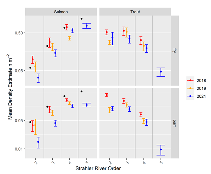
Figure 15 Relationships between Strahler river order and mean estimated densities for salmon and trout, fry and parr obtained by post-stratifying the NEPS data. Coloured points and error bars indicate different survey years. Black points (salmon only) indicate the benchmark for each river order in 2021. Note that plots contain all data collected under NEPS 2021, including strata above barriers on the Forth and Shin that will reduce mean density estimates for salmon relative to 2018 and 2019 surveys.

Inter-annual variability in salmonid densities and status

At the national scale, salmon fry densities were higher in 2021 than 2019, but lower than 2018 (Fig. 16). Parr densities in 2021 were substantially lower than previous surveys and appeared to show a downward trend. Fry densities were above the national benchmark in 2021 and classified as Grade 1. Parr densities were significantly below the benchmark and as such were classified as Grade 3. The overall 2021 classification at a national scale was therefore Grade 2. At a national scale, the densities of trout fry and parr declined across years.

There was considerable regional variability in the abundance of salmon and trout between years (Fig. 17). This spatio-temporal variability in abundance was reflected in similarly complex patterns of variability in NEPS Grades (Fig. 18). However, the consistent downward trend in parr densities observed at the national scale was evident in declining Grades for parr across much of the country, with better performing regions (Grade 1) becoming constrained to the north by 2021.

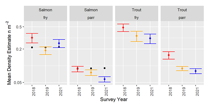
Figure 16 Comparison of juvenile trout and salmon, fry and parr densities between years. Coloured points and error bars indicate mean density estimates. Black points for salmon indicate the national benchmark. Data from NEPS 2021 was post-stratified to provide a sample frame that was broadly consistent with 2018-19 NEPS surveys. Small differences to the benchmark between years reflect changes to sample frame that were not possible to resolve.

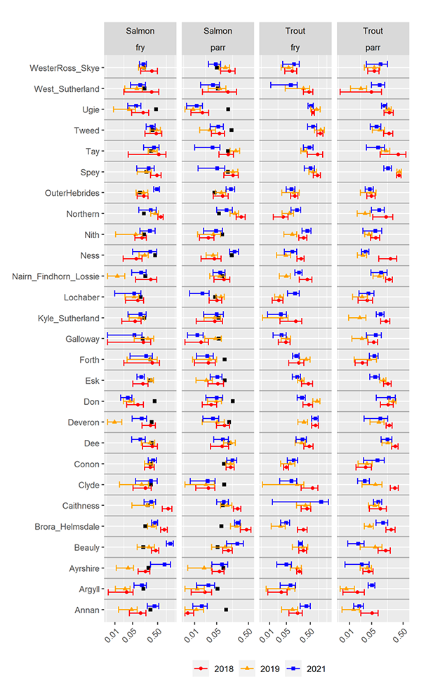
Figure 17. Comparison of observed salmon and trout, fry and parr densities across years. Black circles indicate the benchmarks for salmon. Data from NEPS 2021 were made comparable with data from previous years using post-stratification.

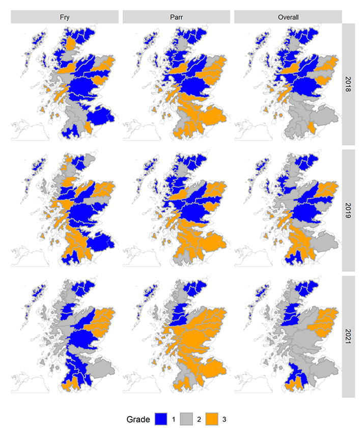
Figure 18 Inter-annual variability in the status (Grades) of salmon fry, parr and the combination of lifestages between NEPS surveys. Data from NEPS 2021 were post-stratified to harmonise between years and allow comparison for common regions and sample frames (Strahler order 2-4 rivers).

Assessing the status of Special Areas of Conservation (SACs) for salmon

There was considerable variability in the estimates of mean salmon densities, benchmark and NEPS grades between SAC rivers (Fig. 19). Only half of the SACs were considered to be in Favourable Condition. Of these, only the River Naver and Mallart Water received a NEPS Grade 1 assessment in every year, with the Spey, Tay and Dee receiving a Grade 1 assessment in two of the three years (Table 1). The River Teith received a NEPS Grade 3 assessment in all years while the River Moriston received a Grade 3 assessment in two of the three years.

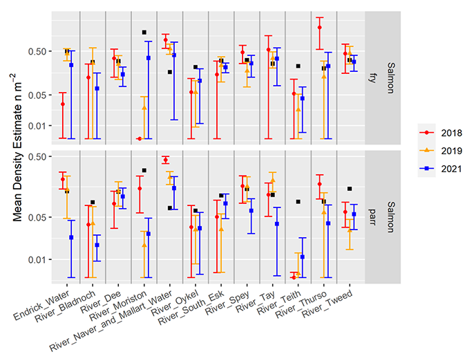
Figure 19 Estimated mean densities (with associated uncertainty) of salmon fry and parr in Special Areas of Conservation (SACs). Data are shown only for SACs with a minimum of five samples in each NEPS sampling year. Black circles indicate the benchmarks for salmon. Data from NEPS 2021 was harmonised with data from previous years by post-stratifying data where necessary.

Table 1 Proposed site condition assessments for SACs based on NEPS data.

SAC	Grade 2018	Grade 2019	Grade 2021	Condition	Fry Trend	Parr Trend	Overall Trend
Endrick	2	1	3	Unfavourable	No Change	Declining	Declining
Bladnoch	2	2	3	Unfavourable	No Change	No Change	No Change
Dee	1	1	2	Favourable	Declining	No Change	Declining
Moriston	2	3	3	Unfavourable	Recovering	No Change	Recovering
Naver & Mallart	1	1	1	Favourable	Declining	Declining	Declining
Oykel	2	2	3	Unfavourable	No Change	No Change	No Change
South Esk	3	2	2	Unfavourable	No Change	No Change	No Change
Spey	1	1	2	Favourable	No Change	Declining	Declining
Tay	1	1	2	Favourable	Declining	No Change	Declining
Teith	3	3	3	Unfavourable	No Change	Recovering	Recovering
Thurso	1	2	2	Favourable	No Change	Declining	Declining
Tweed	2	2	2	Favourable	No Change	No Change	No Change

Relationships between juvenile density, rod catch and NEPS grades

Although NEPS has only run for three years, there were strong positive relationships between rod catch (as a proxy of spawner abundance) and estimates of mean juvenile salmon density at the national scale (Fig. 20). Similar positive relationships can be seen between rod catch (scaled for wetted habitat) and juvenile density at regional scales (Fig. 21), although the greater number of observations and wider range of stock values suggests that habitat may be saturated in some areas (particularly in the north of Scotland) and years. Plotting data in this way ignores spatial variability in habitat quality and carrying capacity which is known to be an important control on abundance (Glover et al., 2018; Malcolm et al., 2019). Nevertheless, accepting these limitations, there is a suggestion that NEPS Grade 1 classifications are likely to be somewhat below maximum carrying capacity.

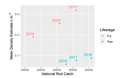
Figure 20 Relationship between salmon rod catch (retained and released) and mean estimated juvenile salmon densities in Strahler order 2-4 rivers. Coloured numbers indicate lagged spawner years (assuming parr are primarily 2 years old).

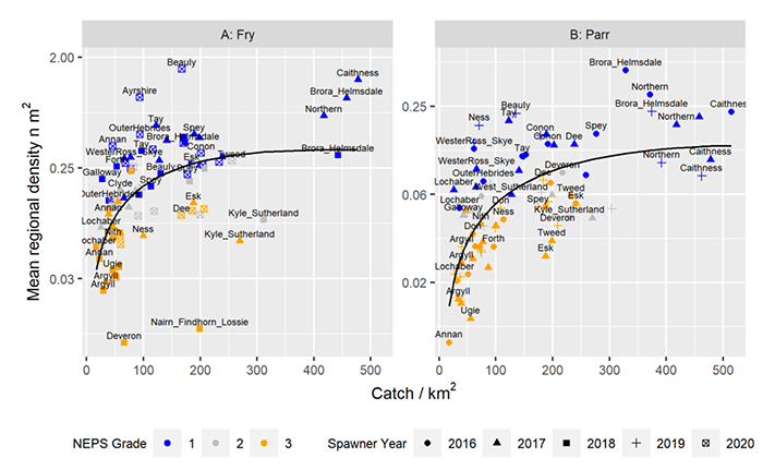
Figure 21 Relationship between salmon rod catch density (catch / km² of accessible river wetted area) and regional estimates of mean juvenile density from Strahler river orders 2-4. Symbols indicate lagged spawner years assuming parr are predominantly 2 years old. Colours indicate NEPS Grades. Black lines show a fitted Ricker stock recruitment relationship.

Spatial Variability in water quality: assessing potential pressures

Spatial variability in water chemistry was broadly consistent between years (Fig. 24, 25, 26). This suggests that the spatially extensive summer spot samples, collected under the low flow conditions, provide a strong basis for characterising within and between river variability in water quality necessary for identifying pressures acting on fish populations.

Total Nitrogen concentrations were highest in urban areas around the central belt, and agricultural areas of the east, north-east and south-west (Fig. 24). Nitrate was the dominant form of nitrogen, although less so in the south-west where organically bound nitrogen likely contributed more substantially than seen elsewhere. As expected, Nitrite and Total Ammonia concentrations were relatively low compared to Nitrate. Nitrite concentrations typically tracked concentrations of Total Nitrogen and Nitrate. Ammonia concentrations were often higher in 2019 than other years but were often patchy in character rather than regionally coherent reflecting potentially localised pollution sources. Nevertheless, higher ammonia concentrations were observed across some north-east and south-western rivers, particularly in 2019.

Total Phosphorous concentrations exhibited spatial patterns that were broadly consistent with Total Nitrogen (Fig. 25). Higher concentrations were observed on the East coast (particularly in the north-east), south-west and central belt. Phosphate, the inorganic form of Phosphorous, was a relatively small component of Total Phosphorous and higher concentrations were generally associated with the north-east and the central belt.

Dissolved Organic Carbon concentrations were typically highest in areas where Nitrogen and Phosphorous concentrations were low reflecting the spatial distribution of organic rich soils that are of lower agricultural value (Fig. 25). Silica concentrations were generally lower in the north-west and higher in the east, particularly the north-east, reflecting regional differences in geology, groundwater contributions and residence times.

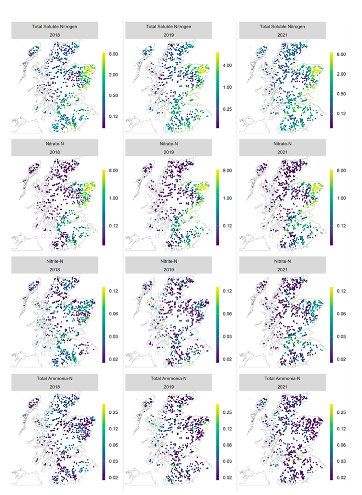
Figure 24 Spatial variability in Nitrogen and Nitrogen compounds between NEPS surveys. Columns relate to NEPS survey years (2018, 2019, 2021), rows relate to chemical determinands. All concentrations are in parts per million (ppm)

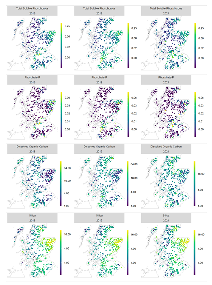
Figure 25 Spatial variability in Total Phosphorous, Phosphate, Dissolved Organic Carbon and Silica between NEPS surveys. Columns relate to NEPS survey years (2018, 2019, 2021), rows relate to chemical determinands. All concentrations are in parts per million (PPM)

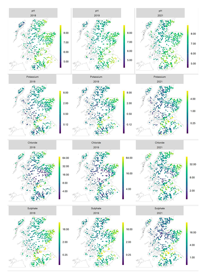
Figure 26 Spatial variability in pH, Potassium, Chloride and Sulphate between NEPS surveys. Columns relate to NEPS survey years (2018, 2019, 2021), rows relate to chemical determinands. All concentrations are in parts per million (ppm) except for pH.

Spatial variability in pH was again consistent with geology, soils and land use. Lower pH values were observed in the west, south-west and Cairngorm mountains, with higher pH on the north-east coast and around the central belt (Fig. 26). Spatial variability in Potassium concentrations largely matched that of nutrients Nitrogen and Phosphorous, potentially indicating a common source from NPK fertilisers. Chloride concentrations were generally higher in coastal areas reflecting marine derived sources. Sulphate concentrations were typically lower in the north-west and higher in the south and east reflecting the influence of both marine derived and anthropogenic sources, the latter being particularly associated with burning of fossil fuels.