Effects of displacement from marine renewable developments on seabirds breeding at the Isle of May

3. Results

3.1. Random prey density

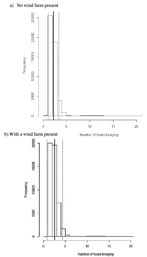
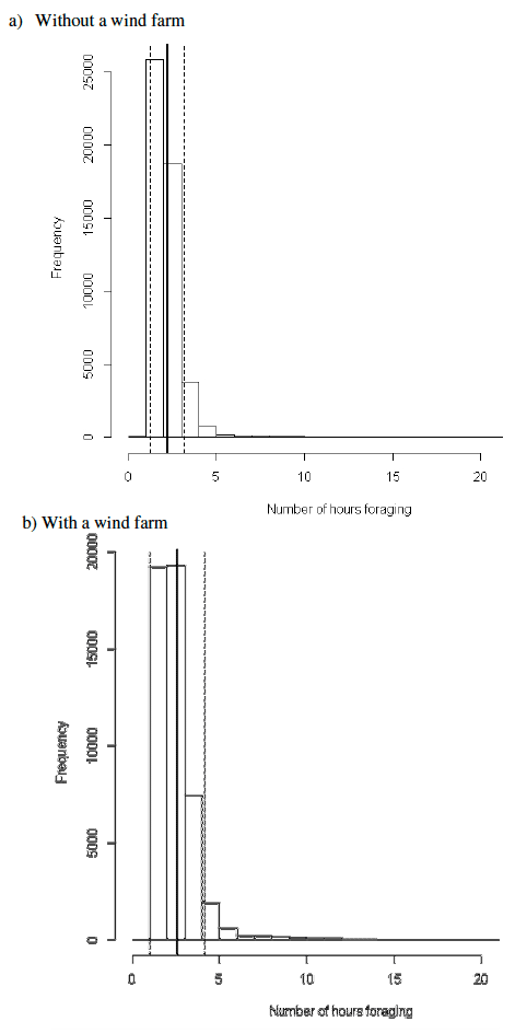
Using a random prey density distribution as an input layer in the simulation model produced a mean distribution of birds per cell across the model space as shown in Figures 6 and 7. In all results, the mean number given is from 50 simulations of 1000 birds in each run. The presence of the wind farm results in a higher density of birds per cell with a particular increase in density of birds on the colony side of the wind farm due to the birds being displaced. The flight and foraging costs increase with increasing distance away from the Isle of May in simulation models both with and without the wind farm (Figures 8 and 9 respectively). The guillemots incur increased average flight costs (Figure 8) and foraging costs (Figure 9) when the wind farm is present. The foraging costs for birds are higher on the colony side of the wind farm, while the flight and foraging costs are higher on the far side. The higher flight costs in Figure 8 are due to birds having to travel a longer distance. The higher foraging costs in Figure 9 are due to an increase in the number of birds in one location which leads to increased disturbance of prey, increased competition and hence, an increase in foraging time to meet energy requirements. Mean flight and foraging costs with and without the wind farm are presented in Table 1 and Figures 10 and 11 respectively.

Table 1. The mean flight and foraging costs for guillemots from the simulations under the three scenarios tested. The summary results are from 50 simulations of 1000 birds.

		Wind farm absent	Wind farm present
Type of Cost	Scenario	Mean cost /hours (± S.D.)	Mean cost /hours (± S.D.)
Flight	Random prey	1.18 (± 0.60)	1.60 (±0.67)
	Clustered prey	1.15 (± 0.67)	1.54 (±0.66)
	Increased interference coefficient	1.18 (± 0.61)	1.57 (±0.66)
Foraging	Random prey	2.19 (± 0.96)	2.58 (± 1.57)
	Clustered prey	2.05 (± 0.85)	2.37 (± 1.16)
	Increased interference coefficient	2.21 (± 1.15)	2.55 (± 1.81)

When the wind farm was not present, the number of birds which do not meet their energy requirements was 1.82 (±3.86) individuals (0.18%). When the wind farm was present, 4.46 (± 7.19) guillemots could not meet their energy requirements (0.46%). The mean number of birds that were displaced by the wind farm was 100.66 (± 28.00) individuals (10.07%). The mean number of birds which incurred additional costs on their outward journey was 43.22 (±10.68) individuals and 45.18 (± 11.18) individuals incurred additional costs on their return journey (4.32% and 4.52% respectively).

Figure 6. The mean number of guillemots within each cell of the simulation model using a random prey density distribution from 50 simulations with a) no wind farm and b) with a wind farm. The scale bars are the number of guillemots per cell and the grey areas indicate land. The hollow polygon indicates the wind farm position. Northings and Eastings are in British National Grid reference system.

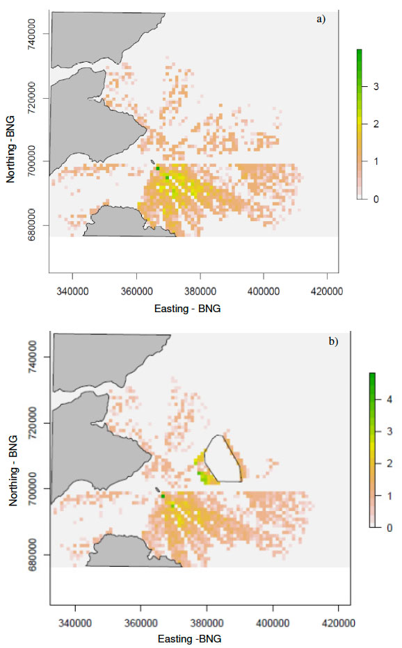
Figure 7. The standard deviation of the mean number of guillemots within each cell from 50 simulations with a random prey density distribution: a) no wind farm and b) with a wind farm. The scale bars are the number of guillemots per cell and the grey areas indicate land. The white polygon indicates the wind farm position. Northings sand Eastings are in the British National Grid ( BNG) reference system.

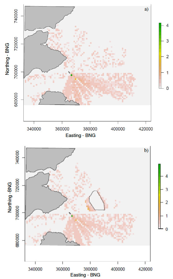
Figure 8. The mean flight cost incurred at each cell after 50 simulations of the model with a random prey density distribution layer and with a) no wind farm and b) with a wind farm present. The scale bars are the number of hours spent in flight and the grey areas indicate land. The hollow polygon indicates the wind farm position. Northings sand Eastings are in the British National Grid ( BNG) reference system.

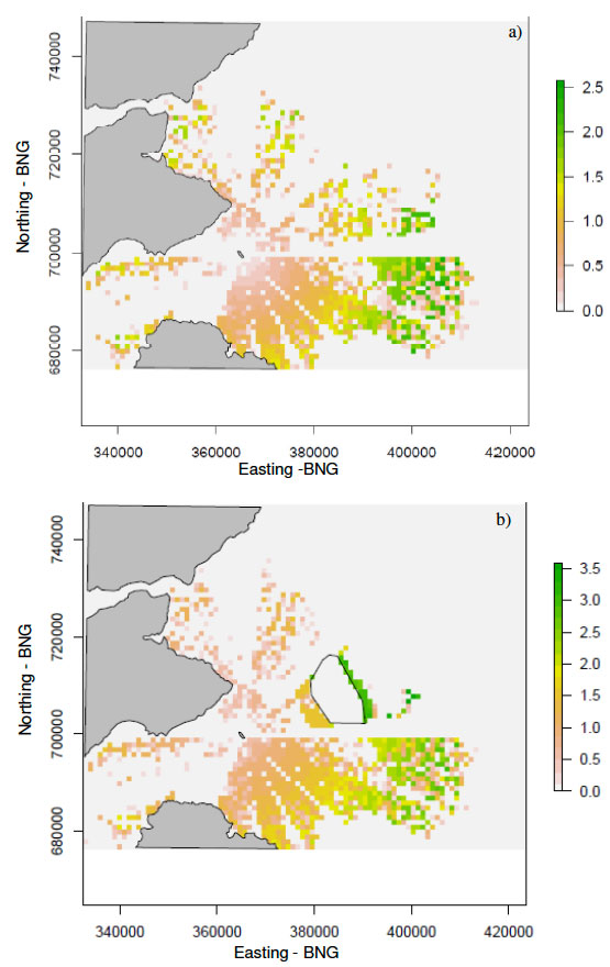
Figure 9. The mean foraging cost incurred at each cell after 50 simulations of the model with a random prey distribution layer and with a) no wind farm and b) with a wind farm present. The scale bars are the number of hours spent foraging and the grey areas indicate land. The white polygon indicates the wind farm position. Northings and Eastings are in the British National Grid ( BNG) reference system.

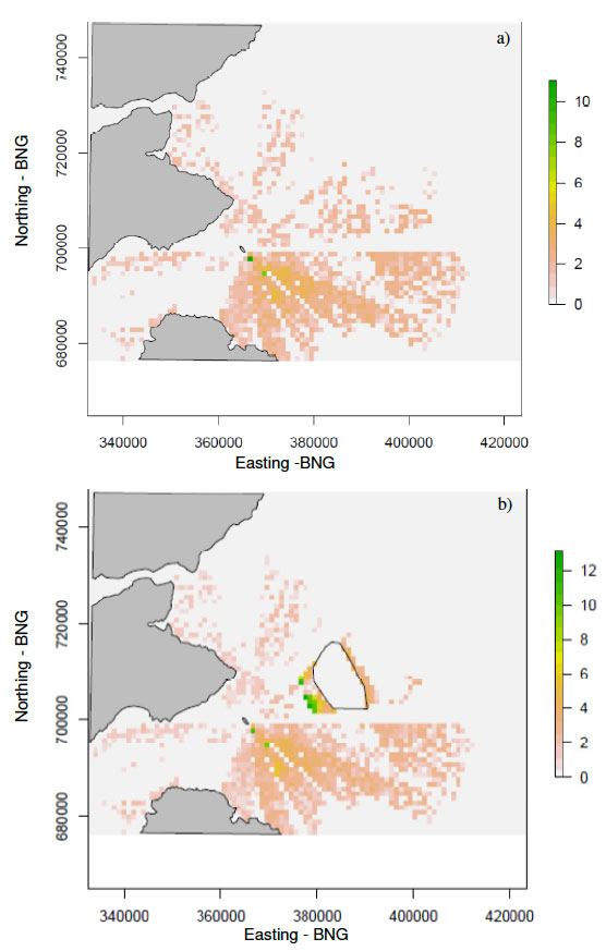
Figure 10. The distribution of flight costs incurred for 50 simulations of 1000 birds with a random prey density layer: a) without a wind farm present and b) with a wind farm present. The bold line indicates the mean flight cost in hours and the dashed lines are the ± standard deviations.

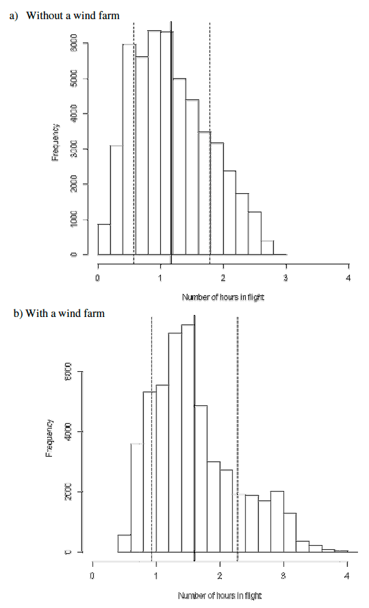
Figure 11. The distribution of foraging costs incurred for 50 simulations of 1000 guillemots with a random prey density layer: a) without a wind farm present and b) with a wind farm present. The bold line indicates the mean flight cost in hours and the dashed lines are the ± standard deviations.

3.2. Clustered prey

Using a more clustered prey density distribution that mimics the shoaling behaviour of forage fish targeted by guillemots as an input layer in the simulation model, produced a mean distribution of birds across the model space as shown in Figures 12 and 13. In all results, the mean number given is from 50 simulations of 1000 birds in each run. Compared to the random prey density distribution model output, there is an increase in the number of birds sharing each location (Figures 12 and 13). The presence of the wind farm results in a higher density of birds per cell with particular increase in density on the colony side of the wind farm due to the birds being displaced. The flight and foraging costs increase with increasing distance away from the Isle of May in simulation models both with and without the wind farm (Figure 14 and Figure 15 respectively). The higher flight costs in Figure 14 are due to birds having to travel a longer distance. The higher foraging costs in Figure 15 are due to an increase in the number of birds in one location which leads to increased disturbance of prey, increased competition and hence, an increase in foraging time to meet energy requirements. The frequency distribution of flight costs and foraging costs for the guillemots are in Figures 16 and 17 and the flight and foraging costs are summarised in Table 1.

When no wind farm is present, the mean number of birds which do not meet their energy requirements was 6.76 (±3.93) individuals (0.68%). When the wind farm was present, 7.66 (± 3.93) guillemots could not meet their energy requirements (0.77%). The mean number of birds that were displaced by the wind farm was 103.34 (± 29.65) individuals (10.33%). The mean number of birds which incurred additional costs on their outward journey and return journey were both 15.10 (±5.72) individuals (1.51%).

Compared to the cost results for the random prey density distribution, the mean flight costs and mean foraging costs were marginally lower when a clustered prey density distribution was used. The presence of the wind farm caused an increase in the mean flight and foraging cost for the clustered prey distribution scenario.

Figure 12. The mean number of guillemots within each cell of the simulation model using a clustered prey density map from 50 simulations with a) no wind farm and b) with a wind farm. The scale bars are the number of guillemots per cell and the grey areas indicate land. The hollow polygon indicates the wind farm position. Northings and Eastings are in the British National Grid ( BNG) reference system.

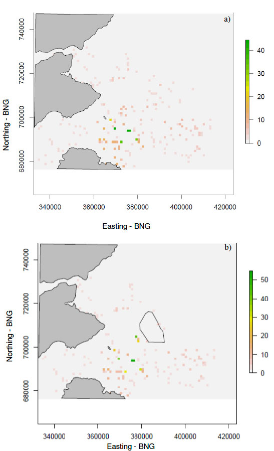
Figure 13. The standard deviation of the mean number of guillemots within each cell from 50 simulations with a clustered prey density distribution: a) no wind farm and b) with a wind farm. The scale bars are the number of guillemots per cell and the grey areas indicate land. The hollow polygon indicates the wind farm position. Northings and Eastings are in the British National Grid ( BNG) system.

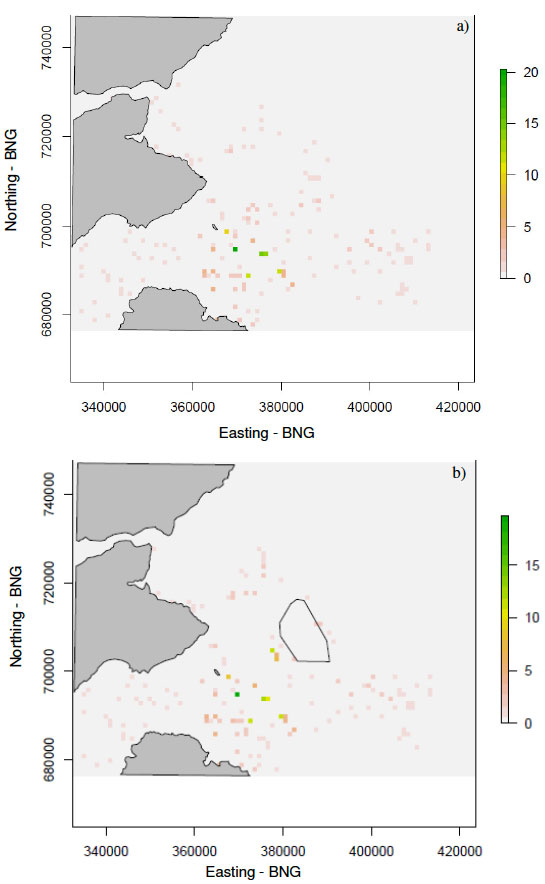
Figure 14. The mean flight cost incurred at each cell after 50 simulations of the model with a clustered prey density distribution layer and with a) no wind farm and b) with a wind farm present. The scale bars are the number of hours in flight and the grey areas indicate land. The hollow polygon indicates the wind farm position. Northings and Eastings are in the British National Grid ( BNG) reference system.

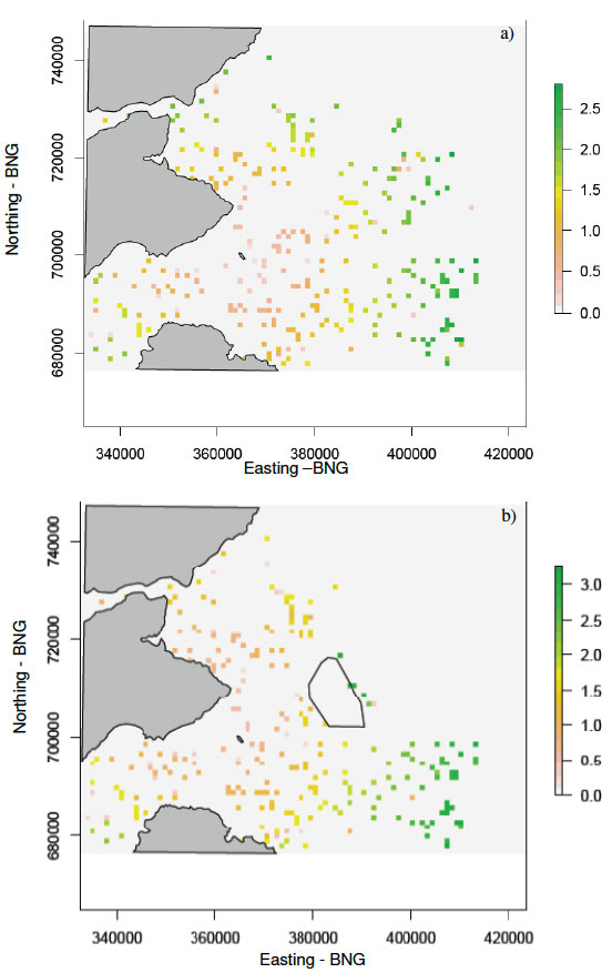
Figure 15. The mean foraging cost incurred at each cell after 50 simulations of the model with a clustered prey distribution layer and with a) no wind farm and b) with a wind farm present. The scale bars are the number of hours spent foraging and the grey areas indicate land. The hollow polygon indicates the wind farm position. Northings and Eastings are in the British National Grid ( BNG) reference system.

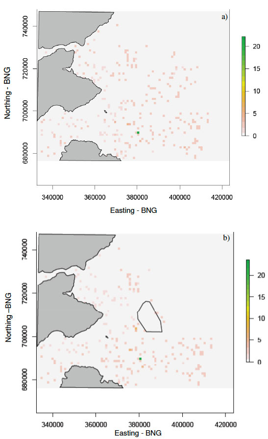
Figure 16. The distribution of flight costs incurred for 50 simulations of 1000 birds with a clustered prey density layer: a) without a wind farm present and b) with a wind farm present. The bold line indicates the mean foraging cost in hours and the dashed lines are the ± standard deviations.

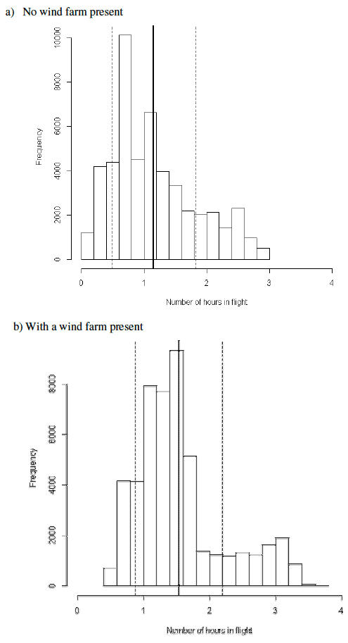
Figure 17. The distribution of foraging costs incurred for 50 simulations of 1000 guillemots with a clustered prey density layer: a) without a wind farm present and b) with a wind farm present. The bold line indicates the mean foraging cost in hours and the dashed lines are the ± standard deviations.

3.3. Increased Interference Coefficient

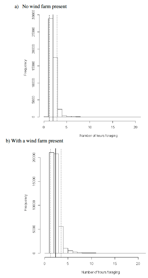
The simulation using an increased interference coefficient in the simulation model produced a mean distribution of birds per cell across the model space as shown in Figures 18 and 19. In all results, the mean number given is from 50 simulations of 1000 birds in each run. Compared to the random prey density distribution model output, there is an increase in the number of birds sharing each location (Figures 18 and 19). The presence of the wind farm results in a higher density of birds per cell particularly on the colony side of the wind farm due to the birds being displaced. Flight and foraging costs increase with increasing distance away from the Isle of May in simulation models both with and without the wind farm (Figure 20 and 21 respectively). The foraging cost for guillemots are higher on the colony side of the wind farm, but the flight and foraging costs are higher on the far side of the wind farm. The higher flight costs in Figure 20 are due to birds having to travel a longer distance. The higher foraging costs in Figure 21 are due to an increase in the number of birds in one location which leads to increased disturbance of prey, increased competition and hence, an increase in foraging time to meet energy requirements. The frequency distribution of flight costs and foraging costs for the guillemots in the simulation with and without the wind farm are shown in Figures 22 and 23. The flight and foraging costs for simulations both with and without a wind farm are summarized in Table 1.

With no wind farm, the mean number of birds which do not meet their energy requirements was 2.40 (±5.15) individuals (0.24%). When the wind farm was present, 5.86 (± 7.07) individuals could not meet their energy requirements (0.59%). The mean number of birds displaced by the wind farm was 83.84 (± 27.84) individuals (8.38%). The mean number of birds incurring additional costs was 38.02 (± 9.69) individuals on the outward journey and 39.40 (±10.16) individuals on their return journey (3.80% and 3.94% respectively).

The increased interference coefficient scenario produced similar flight costs to the scenario with a lower interference coefficient. With no wind farm, the mean number of hours spent foraging is greater with an increased interference coefficient, but when the wind farm is present there is no difference in the mean number of hours spent foraging.

Figure 18. The mean number of guillemots within each cell of the simulation model using a random prey density map and a high interference coefficient from 50 simulations with a) no wind farm and b) with a wind farm. The scale bars are the number of guillemots per cell and the grey areas indicate land. The hollow polygon indicates the wind farm position. Northings and Eastings are in the British National Grid ( BNG) reference system.

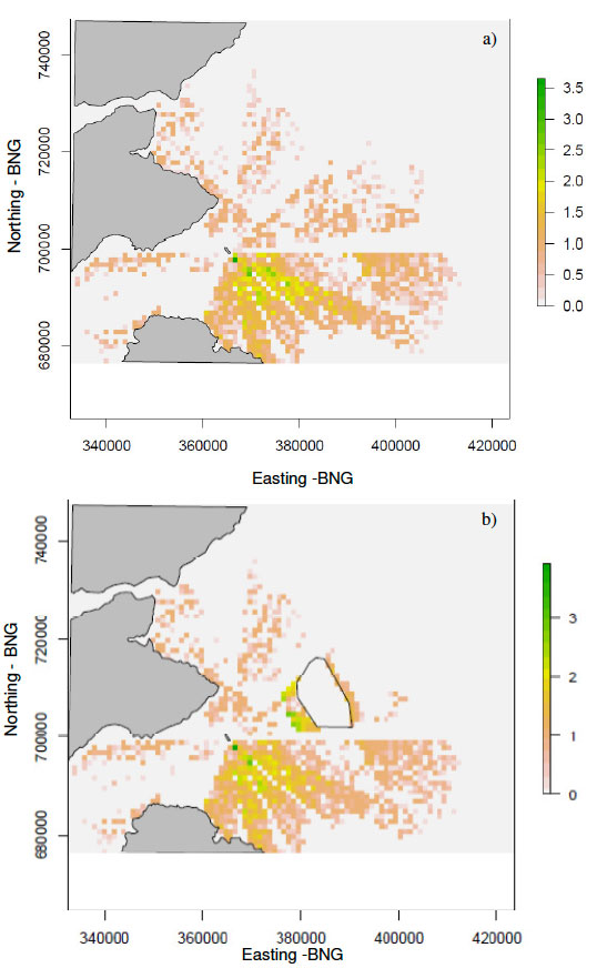
Figure 19. The standard deviation of the mean number of guillemots within each cell from 50 simulations with a random prey density distribution and an increased interference coefficient: a) no wind farm and b) with a wind farm. The scale bars are the number of guillemots per cell and the grey areas indicate land. The hollow polygon indicates the wind farm position. Northings and Eastings are in the British National Grid ( BNG) reference system.

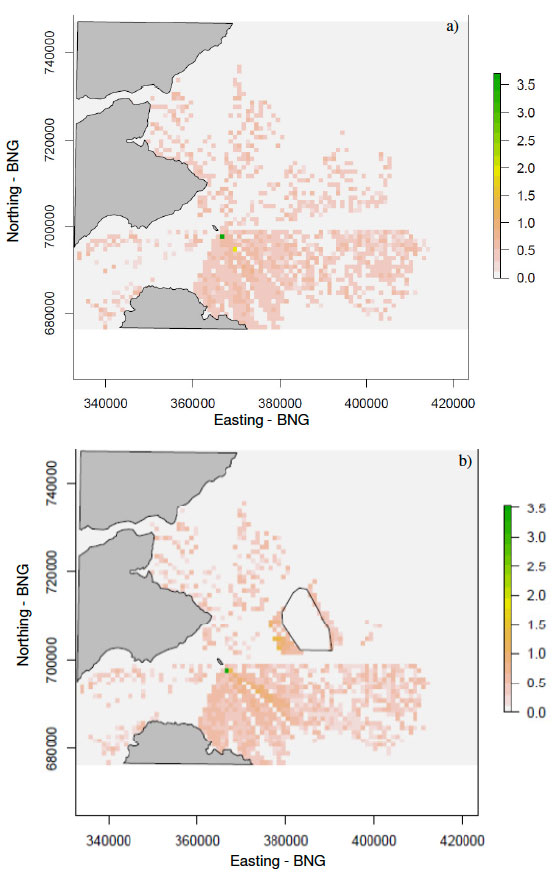
Figure 20. The mean flight cost incurred at each cell after 50 simulations of the model with a random prey density distribution layer, an increased interference coefficient and with a) no wind farm and b) with a wind farm present. The scale bars are the number of hours in flight and the grey areas indicate land. The hollow polygon indicates the wind farm position. Northings and Eastings are in the British National Grid ( BNG) reference system.

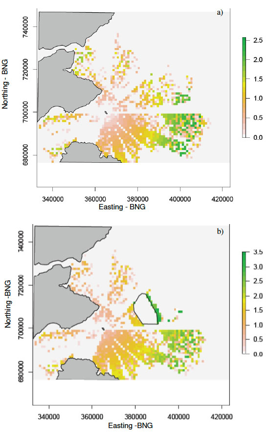
Figure 21. The mean foraging cost incurred at each cell after 50 simulations of the model with a clustered prey distribution layer and with a) no wind farm and b) with a wind farm present. The scale bars are the number hours spent foraging and the grey areas indicate land. The hollow polygon indicates the wind farm position. Northings and Eastings are in the British National Grid ( BNG) reference system.

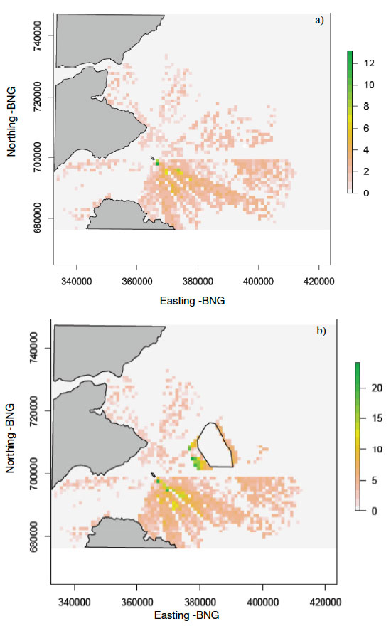
Figure 22. The distribution of flight costs incurred for 50 simulations of 1000 birds with a random prey distribution layer and an increased interference coefficient: a) without a wind farm present and b) with a wind farm present. The bold line indicates the mean flight cost in hours and the dashed lines are the ± standard deviations.

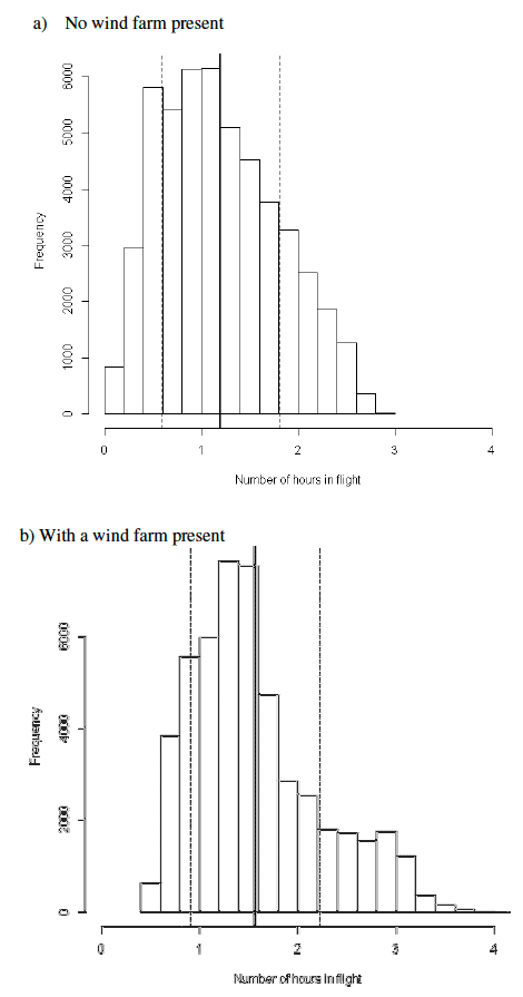
Figure 23. The distribution of foraging costs incurred for 50 simulations of 1000 guillemots with a random prey distribution layer and an increased interference coefficient: a) without a wind farm present and b) with a wind farm present. The bold line indicates the mean foraging cost in hours and the dashed lines are the ± standard deviations.