Feasibility of extending SeabORD to the entire breeding season: study

Extensions

Task 1. Extending SeabORD to entire breeding season for common guillemot, razorbill, Atlantic puffin, black-legged kittiwake and other key species

Key parameters of interest

In order to extend SeabORD to the entire breeding season it is necessary to understand how individuals engage in key behaviours, access resources and interact with one another during each of the remaining breeding phases (pre-laying, incubation and post-fledging). These key factors of interest fall into several broad ecological and behavioural categories:

1) At-sea distribution and habitat use

2) Time-activity budget

3) Foraging trip characteristics

4) Body mass change in adults

5) Colony and nest attendance patterns

For each breeding phase, we identified key parameters within each of these categories that need to be quantified in order to successfully develop individual-based simulations of behaviour and its fitness and population-level consequences (Table 1). We then assessed the availability of data that would be needed to estimate these parameters for each species, focussing mainly on the UK and Ireland. Three main types of data were considered: 1) data obtained from tracking devices deployed on individual birds. These included mainly GPS loggers but also geolocation-immersion loggers (GLS), platform terminal transmitters (PPT) and time-depth recorders (TDR); 2) data obtained from boat-based and aerial at-sea surveys; 3) data obtained from monitoring carried out at the breeding colonies.

Table 1: Key parameters relevant to the extension of SeabORD to the entire breeding season. UD: utilisation distribution; PreLay: pre-laying; Inc: incubation; PostFl: post-fledging.

Category	Parameter	Breeding phase
Distribution	at-sea locations/UDs	PreLay, Inc, PostFl
Habitat	habitat association	PreLay, Inc, PostFl
Time-activity budget	time allocation to flight/foraging/resting/colony	PreLay, Inc, PostFl
Foraging trip characteristics	trip duration foraging site fidelity	PreLay, Inc, PostFl PreLay, Inc, PostFl
Adult body mass	mean mass trend in mass	PreLay, Inc, PostFl PreLay, Inc, PostFl
Colony attendance	arrival date nest attendance departure date	PreLay PreLay, Inc, PostFl PostFl
Length of breeding phase	start and end date	PreLay, Inc, PostFl

Species summaries

Black-legged kittiwake

The kittiwake is a relatively well-studied species with data available from tracking, at-sea surveys and colony monitoring, from multiple years and breeding sites in the UK. Availability of data for the different parameters for each breeding phase is summarised in Table 2; full breakdown of tracking data by breeding colony is provided in Table 3.

For the pre-laying period, data on at-sea distributions are available mainly from at-sea surveys, reflecting the challenges of capturing birds and deploying tracking devices before breeding has initiated. At-sea surveys, however, record locations of both breeding and non-breeding individuals so caution is needed in using these data to determine the distribution of breeders. The most comprehensive source of at-sea survey data for UK waters is the European Seabirds at Sea (ESAS) database which contains data from the NE Atlantic and the North Sea since 1980 (Reid & Camphuysen 1998). At-sea survey data are also collected as part of environmental impact assessments for proposed offshore renewable developments and may be possible to obtain subject to permission from the developers. Geolocation data exist from the colonies at the Isle of May and Bempton Cliffs, however their utility for quantifying at-sea distribution during the breeding season is very limited due to the large error in location estimates (ca.185km). A recent study by Waggitt et al. (2020) developed species distribution models (including ones for kittiwake) using ESAS and environmental data, providing some useful information on habitat association. Furthermore, Wakefield et al (2017) identified important habitat features for kittiwakes and three other species during chick-rearing. Although the study focused on a different breeding phase, the findings may provide useful insight into key habitats that are potentially important during other breeding phases too. Estimates of daily time spent in key behaviours could potentially be derived from immersion (wet/dry) and temperature data recorded by the geolocators deployed on the Isle of May and Bempton Cliffs. However obtaining information on foraging trip characteristics (trip duration and particularly foraging site fidelity) would be challenging as these parameters are commonly derived from GPS data which are lacking for this breeding phase. As part of UKCEH's long-term study on the Isle of May, body mass of pre-laying kittiwakes has been recorded over a number of years so cross-sectional data exist from which both mean mass and change in mass can be derived. Information on arrival dates, colony attendance and length of the pre-laying period could be obtained from geolocation data.

For the incubation period, GPS tracking data are available from a number of UK colonies (Table 3) which would allow determining at-sea distributions, time-activity budgets as well as foraging trip duration and site fidelity. GPS data, in combination with environmental data could be used also for investigating habitat association at a finer scale, whereas broader-scale information is available from Waggitt et al (2020). An estimate of mean adult body mass during incubation could be obtained for several UK colonies monitored by RSPB and UKCEH and cross-sectional data on body mass change exists for the Isle of May. Information on nest attendance and length of the incubation period is available for the Isle of May.

For the post-fledging period, similarly to pre-laying, at-sea distributions and habitat association could be investigated using at-sea survey data, and time-activity budget could be estimated using activity and temperature data from geolocators, but deriving foraging trip characteristics would very difficult due to the lack of GPS data. Limited data on adult body mass and colony attendance is available for the Isle of May, and departure dates and length of the post-fledging period could be derived from geolocation data.

Table 2: Data availability for key parameters for each of the breeding phases in kittiwakes. Data types: AS: at-sea survey; GPS: global positioning system; GLS: geolocation; MON: monitoring. NA: not applicable; - not available.

Parameter	Pre-laying	Incubation	Post-fledging
at-sea locations/UDs	AS	AS GPS	AS
habitat association	AS*	AS*	AS*
time allocation to flight/foraging/resting/colony	GLS	GPS GLS	GLS
trip duration	-	GPS	-
foraging site fidelity	-	GPS	-
mean mass	MON	MON	MON
trend in mass	MON	MON	-
arrival date	GLS	NA	NA
nest/colony attendance	MON	MON	MON
departure date	NA	NA	GLS
start and end date	MON/GLS	MON	MON/GLS

* Species distribution models developed using AS data (Waggitt et al. 2020).

Table 3: UK breeding colonies at which kittiwakes were tracked using GPS loggers or geolocators and total sample sizes of individuals followed in each breeding phase (all years combined).

Breeding colony	Pre-laying		Incubation		Post-fledging
	N GPS	N GLS	N GPS	N GLS	N GPS	N GLS
Bempton Cliffs	0	17	19	17	0	17
Bullers of Buchan	0	0	3	0	0	0
Copinsay	0	0	1	0	0	0
Coquet	0	0	10	0	0	0
Colonsay	0	0	14	0	0	0
Fair Isle	0	0	4	0	0	0
Filey	0	0	5	0	0	0
Fowlsheugh	0	0	19	0	0	0
Isle of May	0	168	51	168	0	168
Muckle Skerry	0	0	13	0	0	0
Puffin Island	0	0	21	0	0	0
Rathlin	0	0	5	0	0	0
St Abbs	0	0	24	0	0	0
St Agnes	0	0	1	0	0	0
St Martin	0	0	5	0	0	0
Whinnyfold	0	0	6	0	0	0

Common guillemot

Availability of data for key parameters for each breeding phase in guillemots is summarised in Table 4 and breakdown of tracking data by breeding colony is presented in Table 5.

For the pre-laying and post-fledging period, data on at-sea distributions are available mainly from at-sea surveys. Information on habitat association is provided in Waggitt et al. (2020) who have developed species distribution models and monthly predicted density maps for key seabird species (including the guillemot) based on at-sea survey and environmental data. Year-round geolocation-immersion data exist for several UK colonies (Table 5), from which estimates of time-activity budgets could be derived. Furthermore, using such data combined with TDR data Dunn at al. (2020) have estimated year-round activity budgets, energy expenditure and colony attendance for Isle of May guillemots. Body mass during the pre-laying phase has been recorded on the Isle of May in multiple years but no mass data are available for the post-fledging period. Information on arrival dates, colony attendance and length of these two breeding phases could be obtained from colony monitoring and geolocation immersion data.

For the incubation period, GPS tracking data are available from a number of colonies monitored by the RSPB (Table 5). These data could be used to determine at-sea distributions, time-activity budgets as well as foraging trip duration and site fidelity. The GPS data, in combination with information on environmental covariates could be used also to investigate habitat association. Adult body mass has been measured in a sample of birds at RSPB colonies. Nest/colony attendance information is available for the Isle of May.

Table 4: Data availability for key parameters for each of the breeding phases in guillemots. Data types: AS: at-sea survey; GPS: global positioning system; GLS: geolocation; TDR: time-depth; MON: monitoring. NA: not applicable; - not available.

Parameter	Pre-laying	Incubation	Post-fledging
at-sea locations/UDs	AS	AS GPS	AS
habitat association	AS*	AS*	AS*
time allocation to flight/foraging/resting/colony	GLS+TDR**	GPS GLS+TDR**	GLS+TDR**
trip duration	-	GPS	-
foraging site fidelity	-	GPS	-
mean mass	MON	MON	-
trend in mass	-	-	-
arrival date	MON, GLS	NA	NA
nest/colony attendance	MON	MON	MON
departure date	NA	NA	MON, GLS
start and end date	MON, GLS	MON	MON, GLS

* Species distribution models developed using AS data (Waggitt et al. 2020); ** activity budgets estimated by Dunn et al (2020)

Table 5: UK breeding colonies at which guillemots were tracked using GPS loggers or geolocators and total sample sizes of individuals followed in each breeding phase (all years combined).

Breeding colony	Pre-laying		Incubation		Post-fledging
	N GPS	N GLS	N GPS	N GLS	N GPS	N GLS
Bullers of Buchan	0	0	2	0	0	0
Canna	0	60	0	60	0	60
Copinsay	0	0	1	0	0	0
Colonsay	0	24	30	24	0	24
East Caithness	0	51	0	51	0	51
Fair Isle	0	0	15	0	0	0
Foula	0	13	0	13	0	13
Isle of May	0	160+	0	160+	0	160+
Lunga	0	0	3	0	0	0
Puffin Island	0	8	3	8	0	8
Shiants	0	0	1	0	0	0
Treshnish	0	14	0	14	0	14
Whinnyfold	0	54	1	54	0	54

Razorbill

Data availability for the key parameters for each breeding phase in razorbills is very similar to that in guillemots although some of the colonies where birds have been tracked differ in the two species (Table 6, Table 7). Also, time-activity budgets have not been estimated for razorbills (and to our knowledge TDR loggers have not been deployed in combination with GLS loggers in this species), however there is a potential to derive activity budgets using geolocation-immersion data only.

Table 6: Data availability for key parameters for each of the breeding phases in razorbills. Data types: AS: at-sea survey; GPS: global positioning system; GLS: geolocation; MON: monitoring. NA: not applicable; - not available.

Parameter	Pre-laying	Incubation	Post-fledging
at-sea locations/UDs	AS	AS GPS	AS
habitat association	AS*	AS*	AS*
time allocation to flight/foraging/resting/colony	GLS	GPS GLS	GLS
trip duration	-	GPS	-
foraging site fidelity	-	GPS	-
mean mass	-	MON	-
trend in mass	-	-	-
arrival date	MON, GLS	NA	NA
nest/colony attendance	MON	MON	MON
departure date	NA	NA	MON, GLS
start and end date	MON, GLS	MON	MON, GLS

* Species distribution models developed using AS data (Waggitt et al. 2020).

Table 7: UK breeding colonies at which razorbills were tracked using GPS loggers or geolocators and total sample sizes of individuals followed in each breeding phase (all years combined).

Breeding colony	Pre-laying		Incubation		Post-fledging
	N GPS	N GLS	N GPS	N GLS	N GPS	N GLS
Bardsey	0	0	9	0	0	0
Canna	0	19	0	19	0	19
Copinsay	0	0	6	0	0	0
Colonsay	0	1	15	1	0	1
East Caithness	0	21	0	21	0	21
Fair Isle	0	11	56	11	0	11
Farne Islands	0	4	0	4	0	4
Flannans	0	0	1	0	0	0
Isle of May	0	50+	0	50+	0	50+
Lunga	0	0	7	0	0	0
Muckle Skerry	0	0	16	0	0	0
Orkney	0	14	0	14	0	14
Puffin Island	0	0	24	0	0	0
Shiants	0	13	4	13	0	13
Swona	0	0	7	0	0	0
Treshnish	0	12	0	12	0	12
Whinnyfold	0	10	0	10	0	10

Atlantic puffin

Availability of data for key parameters for each breeding phase in puffins is summarised in Table 8.

For all three breeding phases, data on at-sea distributions are available mainly from at-sea surveys. Puffins are known to be sensitive to device effects and GPS loggers have not been deployed widely as in the other auk species, or outside the chick rearing period. GPS data during chick rearing exist from the Isle of May (n = 59 successful deployments) and small amounts of data may be available from the Farne Islands. As in the other study species, information on habitat association based on at-sea survey and environmental data is provided in Waggitt et al. (2020). Year-round geolocation-immersion data have been collected as part of long-term studies at two UK colonies: Isle of May (n = 145+) and Skomer (n = 105+, Fayet et al. 2016), which would allow estimating time-activity budgets.

Adult body mass during pre-laying and incubation has been recorded on the Isle of May in multiple years so mean and mass change could be estimated (Harris & Wanless 2012). No mass data, however, are available for the post-fledging period. Information on arrival dates, colony attendance, departure dates, as well as the length of each breeding phase could be obtained from colony monitoring and geolocation-immersion data from the Isle of May and Skomer.

Table 8: Data availability for key parameters for each of the breeding phases in puffins. Data types: AS: at-sea survey; GPS: global positioning system; GLS: geolocation; MON: monitoring. NA: not applicable; - not available.

Parameter	Pre-laying	Incubation	Post-fledging
at-sea locations/UDs	AS	AS	AS
habitat association	AS*	AS*	AS*
time allocation to flight/foraging/resting/colony	GLS	GLS	GLS
trip duration	-	-	-
foraging site fidelity	-	-	-
mean mass	MON	MON	-
trend in mass	MON	MON	-
arrival date	MON, GLS	NA	NA
nest/colony attendance	MON	MON	MON
departure date	NA	NA	MON, GLS
start and end date	MON, GLS	MON	MON, GLS

* Species distribution models developed using AS data (Waggitt et al. 2020).

For species not included in SeabORD so far (European shag, northern gannet, herring gull, lesser black-backed gull and Manx shearwater) we have summarised data availability for the key parameters of interest (Table 1) for all breeding phases, including chick rearing.

European shag

Availability of data for key parameters for each breeding phase in shags is summarised in Table 9 and sample sizes of birds with tracking data by breeding colony are provided in Table 10.

For the pre-laying and post-fledging period, data on at-sea distributions are available mainly from at-sea surveys. Information on habitat association is provided in Waggitt et al. (2020) who have developed species distribution models and monthly predicted density maps for shags and other seabird species, based on at-sea survey and environmental data. The shag is subject of a detailed long-term study by UKCEH, from which there are extensive year-round geolocation-immersion data from Isle of May birds (Table 10). Estimates of time-activity budgets could be obtained from these data, and daily foraging time has already been derived in a previous study (Daunt et al. 2014). Body mass data for these breeding phases are not available. Information on arrival dates, colony attendance and length of these breeding phases could be obtained from colony monitoring and resightings of colour-ringed shags carried out at several colonies as part of a long-term study by UKCEH and the University of Aberdeen.

For the incubation and chick rearing periods, in addition to at-sea survey and geolocation-immersion data, GPS tracking data are available from a number of colonies (Table 10). These could be used to determine at-sea distributions, time-activity budgets, foraging trip duration and site fidelity. Habitat association during chick rearing has been investigated by Wakefield et al. (2017), using GPS tracking and environmental data, and the same approach could be applied to the incubation period. Adult body mass has been measured in a sample of birds at RSPB colonies (incubation) and at RSPB colonies and the Isle of May (chick rearing). Nest/colony attendance information is available for the Isle of May.

Table 9: Data availability for key parameters for each of the breeding phases in shags. Data types: AS: at-sea survey; GPS: global positioning system; GLS: geolocation; MON: monitoring. NA: not applicable; - not available.

Parameter	Pre-laying	Incubation	Chick rearing	Post-fledging
at-sea locations/UDs	AS	AS GPS	AS GPS	AS
habitat association	AS*	AS*	GPS*, AS*	AS*
time allocation to flight/foraging/resting/colony	GLS	GPS GLS	GPS GLS	GLS
trip duration	-	GPS	GPS	-
foraging site fidelity	-	GPS	GPS	-
mean mass	-	MON	MON	-
trend in mass	-	-	MON	-
arrival date	MON	NA	NA	NA
nest/colony attendance	MON	MON	MON	MON
departure date	NA	NA	NA	MON
start and end date	MON	MON	MON	MON

* Species distribution models developed using GPS and AS data (Wakefield et al. 2017, Waggitt et al. 2020).

Table 10: UK breeding colonies at which shags were tracked using GPS loggers or geolocation- immersion loggers and total sample sizes of individuals followed in each breeding phase (all years combined).

Breeding colony	Pre-laying		Incubation		Chick rearing		Post-fledging
	N GPS	N GLS	N GPS	N GLS	N GPS	N GLS	N GPS	N GLS
Annet	0	0	1	0	6	0	0	0
Colonsay	0	0	12	0	41	0	0	0
Copinsay	0	0	7	0	15	0	0	0
Fair Isle	0	0	7	0	11	0	0	0
Great Saltee	0	0	0	0	5	0	0	0
Inchkeith	0	0	0	0	5	0	0	0
Isle of May	0	444	0	444	89+	444	0	444
Lambay	0	0	0	0	20	0	0	0
Lunga	0	0	7	0	11	0	0	0
Muckle Skerry	0	0	7	0	25	0	0	0
Puffin Island	0	0	0	0	60	0	0	0
Rathlin	0	0	0	0	1	0	0	0
Samson	0	0	0	0	6	0	0	0
Sumburgh Head	0	0	0	0	2	0	0	0

Northern gannet

The gannet is one of the relatively well-studied seabird species, with data available from tracking, at-sea surveys and colony monitoring, from multiple breeding sites across the UK and Ireland. Availability of data for the different parameters for each breeding phase is summarised in Table 11; information on sample sizes of tracked individuals by breeding colony is provided in Table 12.

For the pre-laying and incubation periods, data on at-sea distributions are available mainly from at-sea surveys and geolocation. A species distribution model and monthly predicted density maps for gannets have been developed by Waggitt et al. (2020), using at-sea survey and environmental covariates data. Year-round geolocation-immersion data exist for several UK colonies (Table 12), from which estimates of time-activity budgets could be derived. To our knowledge, body mass data for these breeding phases are not available as colonies are commonly visited (and birds captured) during chick rearing. Information on colony arrival dates and colony attendance could be obtained from geolocation-immersion data. In addition, some data for the colony at Bass Rock may be available from monitoring carried out by the Scottish Seabird Centre.

Most GPS/PTT/TDR tracking studies of gannets have been carried out during chick-rearing, therefore at-sea distributions, habitat association, time-activity budgets and foraging trip characteristics can be estimated with greater accuracy for this breeding phase. Both at-sea distributions and habitat use have been investigated as part of previous studies (Wakefield et al. 2013, Grecian et al. 2018). Body mass and nest attendance have been recorded at several colonies where the species is being tracked.

Although less focus has been placed on the post-fledging period, some of the longer GPS/PTT deployments initiated during chick rearing have yielded data during post-fledging too which would allow parameters to do with at-sea distribution, habitat use and activity budgets to be estimated. As with pre-laying and incubation, adult body mass data are lacking. Information on colony attendance and departure dates could be obtained from geolocation-immersion data and GPS data, and for Bass Rock additional monitoring data may be available from the Scottish Seabird Centre.

Table 11: Data availability for key parameters for each of the breeding phases in gannets. Data types: AS: at-sea survey; GPS: global positioning system; PTT: platform terminal transmitter; GLS: geolocation; TDR: time-depth recorder, MON: monitoring. NA: not applicable; - not available.

Parameter	Pre-laying	Incubation	Chick rearing	Post-fledging
at-sea locations/UDs	AS (GLS)	AS (GLS)	AS GPS, PTT	AS GPS, PTT
habitat association	AS*	AS*	GPS*, AS*	AS*
time allocation to flight/foraging/resting/colony	GLS	GLS	GPS, PTT, TDR GLS	GPS, PTT GLS
trip duration	-	-	GPS, PTT	GPS, PTT
foraging site fidelity	-	-	GPS, PTT	GPS, PTT
mean mass	-	-	MON	-
trend in mass	-	-	(MON)	-
arrival date	MON, GLS	NA	NA	NA
nest/colony attendance	MON	MON	MON	MON
departure date	NA	NA	NA	MON, GLS
start and end date	MON, GLS	MON	MON	MON, GLS

* Species distribution models developed using AS data (Waggitt et al. 2020), habitat association from GPS data (Grecian et al 2018).

Table 12: UK and Irish breeding colonies at which gannets were tracked using GPS loggers, platform terminal transmitters or geolocation-immersion loggers and total sample sizes of individuals followed in each breeding phase (all years combined). TBC: to be confirmed whether geolocation-immersion loggers were deployed.

Breeding colony	Pre-laying		Incubation		Chick rearing			Post-fledging
	N GPS	N GLS	N GPS	N GLS	N GPS	N PTT	N GLS	N GPS	N PTT	N GLS
Ailsa Craig	0	TBC	0	TBC	16	0	TBC	0	0	TBC
Bass Rock	0	66+	0	66+	100+	0	66+	0	0	66+
Bempton	0	TBC	0	TBC	10	42	TBC	18	0	TBC
Bull Rock	0	TBC	0	TBC	14	0	TBC	0	0	TBC
Grassholm	0	33+	0	33+	47+	0	33+	0	0	33+
Great Saltee	0	8+	0	8+	35	0	8+	0	0	8+
Lambay	0	TBC	0	TBC	3	0	TBC	0	0	TBC
Little Skellig	0	TBC	0	TBC	9	0	TBC	0	0	TBC
St Kilda	0	TBC	0	TBC	0	21	0	0	2	0
Sule Skerry	0	TBC	0	TBC	2	0	TBC	0	0	TBC

Herring gull

The herring gull has been more extensively studied outside the UK and Ireland, therefore we have included information from non-UK colonies. Availability of data for the different parameters for each breeding phase is summarised in Table 13; information on sample sizes of tracked individuals by breeding colony is provided in Table 14.

Unlike the previous study species, herring gulls at non-UK colonies have been deployed with state of the art GPS-accelerometer-altimeter loggers that remain on the birds year round via a harness attachment. Therefore, although from few colonies (mainly Texel in the Netherlands), data exist that would allow determining at-sea distribution, habitat association, time-activity budgets and foraging trip characteristics for all breeding phases. It is worth noting, however, that this species forages extensively in terrestrial and inter-tidal habitats so use of marine areas may be limited. The tracking data from Texel have recently been used to investigate the links between time-activity budgets, habitat use and foraging site fidelity during incubation (Van Donk et al. 2020). Foraging trip characteristics and habitat use have been studied at colonies in the German Wadden Sea as well (Enners et al. 2018). In the UK, at-sea survey data are available from the ESAS database and a limited amount of GPS tracking data exist from several colonies (Table 14). A species distribution model and monthly predicted density maps have been developed by Waggitt et al. (2020). Body mass measurements are available mainly for the incubation period when birds are captured as part of tracking studies. Timing of colony arrival and departure, and colony attendance could be extracted from GPS data; and limited monitoring data may exist for some of the colonies.

Table 13: Data availability for key parameters for each of the breeding phases in herring gulls. Data types: AS: at-sea survey; GPS: global positioning system; MON: monitoring. NA: not applicable; - not available. Non- UK data included.

Parameter	Pre-laying	Incubation	Chick rearing	Post-fledging
at-sea locations/UDs	AS GPS	AS GPS	AS GPS	AS GPS
habitat association	AS*	GPS*, AS*	GPS*, AS*	AS*
time allocation to flight/foraging/resting/colony	GPS	GPS	GPS	GPS
trip duration	GPS	GPS	GPS	GPS
foraging site fidelity	GPS	GPS	GPS	GPS
mean mass	-	MON	(MON)	-
trend in mass	-	MON	-	-
arrival date	GPS	NA	NA	NA
nest/colony attendance	GPS	GPS	GPS	GPS
departure date	NA	NA	NA	GPS
start and end date	GPS	GPS	GPS	GPS

* Species distribution models developed using AS data (Waggitt et al. 2020), habitat association from GPS data (Van Donk et al. 2020).

Table 14: Breeding colonies in Europe at which herring gulls were tracked using GPS loggers and total sample sizes of individuals followed in each breeding phase (all years combined).

Breeding colony	Pre-laying	Incubation	Chick rearing	Post-fledging
	N GPS	N GPS	N GPS	N GPS
East Caithness	0	5	0	0
Havergate Island	0	6	0	0
Oland, Langeness & Amrum (non-UK)	0	37	13	0
Orford Ness	0	4	0	0
St Ives (urban)	1	4	4	1
Texel (non-UK)	31	31	31	31

Lesser black-backed gull

Similar to the herring gull, this species has been extensively studied outside the UK and Ireland, therefore we have included information from non-UK colonies too. Availability of data for the different parameters for each breeding phase is summarised in Table 15; information on sample sizes of tracked individuals by breeding colony is provided in Table 16.

As with herring gulls, lesser black-backed gulls have been deployed with state of the art GPS-accelerometer-altimeter loggers that remain on the birds year round. Studies have been conducted at a larger number of colonies (both within and outside the UK) compared to herring gulls, therefore detailed data exist that allow determining at-sea distribution, habitat association, time-activity budgets and foraging trip characteristics for all breeding phases (for example, using such data Spelt et al. 2019 investigated time-activity budgets and habitat use in urban-nesting gulls). Timing of colony arrival and departure, and colony attendance could also be extracted from the GPS data. Body mass measurements are available mainly for the incubation period when birds are captured as part of tracking studies.

Table 15: Data availability for key parameters for each of the breeding phases in lesser black-backed gulls. Data types: AS: at-sea survey; GPS: global positioning system; MON: monitoring. NA: not applicable; - not available. Non- UK data included.

Parameter	Pre-laying	Incubation	Chick rearing	Post-fledging
at-sea locations/UDs	AS GPS	AS GPS	AS GPS	AS GPS
habitat association	AS*	GPS*, AS*	GPS*, AS*	AS*
time allocation to flight/foraging/resting/colony	GPS	GPS	GPS	GPS
trip duration	GPS	GPS	GPS	GPS
foraging site fidelity	GPS	GPS	GPS	GPS
mean mass	-	MON	(MON)	-
trend in mass	-	-	-	-
arrival date	GPS	NA	NA	NA
nest/colony attendance	GPS	GPS	GPS	GPS
departure date	NA	NA	NA	GPS
start and end date	GPS	GPS	GPS	GPS

* Species distribution models developed using AS data (Waggitt et al. 2020), habitat association from GPS data (Baert et al. 2018, Spelt et al. 2019).

Table 16: Breeding colonies in Europe at which lesser black-backed gulls were tracked using GPS loggers and total sample sizes of individuals followed in each breeding phase (all years combined). Because not all loggers record for the full duration of the year, there is some uncertainty regarding sample sizes of individuals for which data exist for the pre-laying period. These are presented in brackets.

Breeding colony	Pre-laying	Incubation	Chick rearing	Post-fledging
	N GPS	N GPS	N GPS	N GPS
Bristol (urban)	(11)	11	11	11
Havergate Island	(4)	4	4	4
Orford Ness	18	24	24	24
Ostend (non-UK)	(<6)	6+	6+	6+
Skokholm	20	25	25	25
Texel (non-UK)	19+	51+	51+	51+
Vlissingen (non-UK)	(<31)	31+	31+	31+
Walney	16	24	24	24
Zeebrugge (non-UK)	(<70)	70+	70+	70+

Manx shearwater

Manx shearwaters have been extensively studied at several UK colonies, mainly as part of long-term studies by the University of Oxford. Availability of data for the different parameters for each breeding phase is summarised in Table 17; information on sample sizes of tracked individuals by breeding colony is provided in Table 18.

For the pre-laying and post-fledging period, at-sea distributions could be obtained mainly from at-sea surveys and geolocation loggers (GLS data could potentially be utilised as the species is wide-ranging even during the breeding season). A species distribution model and monthly predicted density maps have been produced by Waggitt et al. (2020). Manx shearwaters are subject of a detailed long-term study by the University of Oxford, from which extensive year-round geolocation-immersion data exist for two colonies (Skomer and Copeland Islands, Table 18). Such data would allow time-activity budgets to be estimated. To our knowledge, body mass data for these breeding phases are not available. Information on arrival dates, colony attendance and length of the breeding phases could be obtained from geolocation-immersion data and colony monitoring.

For the incubation and chick rearing periods, in addition to at-sea survey and geolocation-immersion data, GPS tracking data are available from several colonies; TDR loggers have also been deployed during chick rearing. In combination, these tracking data could be used to determine at-sea distributions, habitat use, time-activity budgets and foraging trip characteristics. Adult body mass has been measured multiple times for tracked individuals, allowing body mass change to be estimated (Gillies et al. 2020). Nest/colony attendance information is likely available for extensively-studied colonies such as Skomer and the Copeland Islands.

Table 17: Data availability for key parameters for each of the breeding phases in Manx shearwaters. Data types: AS: at-sea survey; GPS: global positioning system; GLS: geolocation; MON: monitoring. NA: not applicable; - not available.

Parameter	Pre-laying	Incubation	Chick rearing	Post-fledging
at-sea locations/UDs	AS	AS GPS	AS GPS	AS
habitat association	AS*	AS*	AS*	AS*
time allocation to flight/foraging/resting/colony	GLS	GPS GLS	GPS+TDR GLS	GLS
trip duration	-	GPS	GPS	-
foraging site fidelity	-	GPS	GPS	-
mean mass	-	MON	MON	-
trend in mass	-	MON	MON	-
arrival date	MON, GLS	NA	NA	NA
nest/colony attendance	MON	MON	MON	MON
departure date	NA	NA	NA	MON, GLS
start and end date	MON, GLS	MON	MON	MON, GLS

* Species distribution models developed using AS data (Waggitt et al. 2020).

Table 18: UK and Irish breeding colonies at which Manx shearwaters were tracked using GPS loggers or geolocators and total sample sizes of individuals followed in each breeding phase (all years combined). TBC: to be confirmed whether geolocation-immersion loggers were deployed.

Breeding colony	Pre-laying		Incubation		Chick rearing		Post-fledging
	N GPS	N GLS	N GPS	N GLS	N GPS	N GLS	N GPS	N GLS
Copeland Islands	0	31+	TBC	31+	111	31+	0	31+
Great Blasket	0	0	0	0	18	0	0	0
High Island	0	0	0	0	33	0	0	0
Lundy	0	TBC	0	TBC	18	TBC	0	TBC
Rum	0	0	0	0	14	0	0	0
Skokholm	0	TBC	0	TBC	12	TBC	0	TBC
Skomer	0	108+	TBC	108+	204	108+	0	108+

Recommendations and key knowledge gaps

During incubation, tracking, at-sea survey and monitoring data have been collected for most of the species considered here, often at multiple colonies and/or years, providing good basis for extending SeabORD to this breeding phase.

Much less data exist for the pre-laying and post-fledging phases. Monitoring data for those are limited and tracking data are mainly obtained from geolocation immersion loggers which are generally not of sufficient resolution to investigate distributions and foraging trip characteristics. An exception are the large gull species where higher resolution data have been collected using state-of the art GPS-accelerometer-altimeter technology. The scope for extending SeabORD to these breeding phases is therefore limited.

For the additional species we considered (European shag, northern gannet, herring gull, lesser black-backed gull and Manx shearwater), there is potential for extending SeabORD to the incubation and chick-rearing phases. Substantial amounts of data are available for chick-rearing in particular.

Additional considerations include: 1) use of any data that are not owned by UKCEH and RSPB, or freely available from public repositories, would be subject to permissions from the data owners, therefore access to existing data is not automatically guaranteed; 2) data collation as well as extracting the parameters of interest (particularly to do with habitat association, time-activity budgets and foraging trip characteristics) for the number of species we are considering would be a very substantial undertaking.

Given the limited availability of data in many species, key knowledge gaps are apparent in our understanding of the ecology of seabirds outside the chick-rearing period during the breeding season. Future targeted data collection could focus on filling these knowledge gaps, but will be strongly constrained by feasibility. In particular, obtaining GPS tracking data during the pre-laying, incubation and post-fledging periods will remain a challenge in species not suited to harness attachments until leg-deployed GPS loggers of a size comparable to GLS loggers are available. There will also be significant challenges in increasing data on body mass and condition during these periods because it is not generally possible to catch birds at these times in many species. Data on timing of arrival and departure from and attendance rates at colonies during pre-laying and post-fledging periods could be improved using camera technology, which is seeing an explosion in deployment at seabird colonies at the moment, and MOTUS tags, which are currently under development.

Task 2. Consideration of recommendations on how SeabORD can be further developed to address actions identified in SNH's marine bird impact assessment guidance workshop

Recommendation 33. Further development of SeabORD to include prey distribution data and turbine density/spacing

a) Prey data

SeabORD currently uses prey distribution maps to determine how birds interact with prey resources at their chosen foraging location across their foraging range from the breeding colony. In practice, these are often inferred from bird utilisation distributions derived from GPS tracking data, due to a lack of available data on key seabird prey species. Simulated birds then interact with prey at their chosen foraging location, with a functional response mechanism in the model determining each individual's intake rate and subsequent energy intake rate and energy gained during the foraging bout.

Therefore, SeabORD itself needs no further development to include prey distribution data, rather new synthesis of existing data coupled with new empirical data collection and statistical modelling is required to better quantify the distribution, abundance and availability of key prey species in UK waters throughout the breeding season and other times of the year.

Lesser sandeels (Ammodytes marinus) are the principal prey of most seabird species during the breeding season in the North Sea, including common guillemots, razorbills, Atlantic puffin, northern gannets and black-legged kittiwakes, and we therefore focus this section of the report on this species. However, other prey species are important in the diet of seabirds during the breeding season, notably small clupeids such as sprats (Sprattus sprattus), particularly in more southerly colonies in the North Sea (Anderson et al. 2014), and juvenile gadids in more northerly colonies (Anderson et al. 2014). Moreover, there is evidence that the proportion of sandeel in the diet of chick-rearing seabirds is declining (Wanless et al. 2018), so an important research gap remains for developing fine resolution spatially explicit maps for other prey species.

Inference on spatial prey availability from fish research

At a broad scale, there is evidence for important phenotypic variation across regional populations of lesser sandeel (Ammodytes marinus) in the North Sea (Pedersen et al. 1999, Boulcott et al. 2007, Rindorf et al. 2016, Wright et al. 2019), and spatio-temporal structure in this key prey species will likely affect the quantity and quality of available prey for seabirds breeding in the North Sea across different colony locations (Rindorf et al. 2016) and their subsequent demographics (Frederiksen et al. 2005, Olin et al. 2020). Sandeel habitat preferences have been identified from grab sampling time series in the north-western North Sea (Holland et al. 2005), and subsequently broad habitat areas have been mapped across the whole of the North Sea (Jensen et al. 2011). The limited availability of their preferred substratum means their post-settlement distribution is patchy (Holland et al. 2005). Sandeels are difficult to sample in the water column due to their burying behaviour, and this combined with the patchy distribution of suitable habitat means that regular North Sea acoustic and trawl surveys do not provide tractable or reliable means of mapping sandeel distribution across the North Sea (Jensen et al. 2011), although densities have been estimated using these sources in a few areas (Greenstreet et al. 2006). Consequently, sandeel distribution has tended to be derived indirectly from a range of information sources, including fisheries information (Pedersen et al. 1999), which is known to be problematic (Holland et al. 2005, Moriarty et al. 2020), and estimates for sandeel distribution in the North Sea have most often been limited to spatial mapping of habitat or foraging habitat (Jensen et al. 2011), or area-specific estimates of sandeel population biomass (Greenstreet et al. 2006). More recently, analyses linking the length and condition of sandeels in the North Sea with physical and biological characteristics have enabled the development of spatially explicit maps of sandeel predicted length and condition across the North Sea (Rindorf et al. 2016), albeit at a broad resolution making direct linkage to foraging patterns of individual breeding seabirds difficult.

The most promising research on prey availability for seabirds in the North Sea is currently being developed by Marine Scotland Science, using data on lesser sandeel abundance and sediment from grab surveys to produce a species distribution model to predict the occurrence and density of sandeels in parts of the North Sea (Langton et al. 2021). This predictive distribution model estimates the probability of occurrence and density of sandeels, at a 200m resolution, and will help to refine previous estimates for sandeel availability to predators. The fine resolution of the predictive model for density means model outputs have the potential to be used within individual-based models like SeabORD to derive prey availability at chosen foraging locations of breeding seabirds in the relevant modelled regions (from Shetland to south of the protected sandbanks off Norfolk).

Recent work has highlighted the importance of temperature effects on recruitment of sandeels in the North Sea, identifying the potential for phenological decoupling of sandeel hatching and egg production of its copepod prey (Regnier et al. 2019). Projected warming scenarios for the North Sea indicate an increasing probability of trophic mismatch between sandeels and their prey (Regnier et al. 2019), highlighting the dynamic nature of sandeel distribution and population dynamics under future climate change in this region (Heath et al. 2012). These likely shifts in subsequent prey availability for breeding seabirds indicate the need for more predictive monitoring of sandeel distribution and dynamics over the coming decades to inform predator-prey interactions for protected UK seabird populations and the impact of shifts on interactions with ORDs. Ideally, spatially-explicit predictive maps of sandeel availability for foraging seabirds are needed to drive simulation-based models such as SeabORD.

Inference on spatial prey availability from seabird research

An alternative to utilising direct measurements of prey species to estimate prey availability for seabirds has been to develop estimates derived indirectly from seabird foraging behaviour.

Individual tagging data using devices such as GPS sensors, time-depth-recorders (TDRs) and accelerometers have been used to infer characteristics of foraging activity assumed to be related to prey availability (Boyd et al. 2015, Carroll et al. 2017, Chimienti et al. 2017). Such methods have been used to infer capture attempt rates for foraging razorbills and guillemots from two UK colonies (Chimienti et al. 2017), which could be used to update or validate existing intake rate mechanisms within SeabORD (i.e., the functional response component). The most detailed studies have used multiple sensors with camera technology to record pursuit and catching events, which can then be used to estimate gain functions for foraging seabirds (energy gain versus residence time within a prey patch), but have thus far been restricted to larger species such as penguins (Watanabe et al. 2014) and European shag. Some indirect inferences using TDR data have been attempted for smaller species, suggesting asymptotic rates of gain for foraging razorbills, and asymptotic or linear rates for foraging common guillemots (Chimienti et al. 2017), consistent with the current parameterisation of SeabORD functional responses. Additional research on these foraging characteristics such as pursuit times and capture rates would allow for more sophisticated parameterisation of energy gain within SeabORD, and validation of the existing parameterisations within the model. However, these various indirect methods still then need to be linked to inference about spatial and temporal variation in prey availability for foraging seabirds, and how this may be affected by environmental variation, to develop a stronger link between prey availability and energy gain by foraging seabirds.

At broad scales, early work has demonstrated overlap between spatial patterns of seabird occurrence (ESAS data) and sandeel habitat during the breeding season (Wright and Begg 1997), however spatially explicit mapping of sandeel habitat tends to be restricted to fairly coarse spatial resolution, thereby limiting its applicability to individual-based models such as SeabORD. More recently, joint spatial models have been developed for common guillemot, black‐legged kittiwake, northern gannet and sandeels to estimate joint habitat distribution for predator-prey species by identifying bio/physical covariate correlates (Sadykova et al. 2017). These models used seasonal ESAS data on seabirds at sea and sandeel data from Continuous Plankton Recorder (CPR) surveys, kriged to match covariates across a 7*7km grid (Sadykova et al. 2017). The predicted joint distributions have the potential for use within individual-based models such as SeabORD, although due to having been derived from at-sea survey data, the derived relationships may be less appropriate for breeding birds due the presence of non-breeders within these data.

Recommendations and key knowledge gaps

The most promising improvement for how SeabORD currently incorporates prey availability is the soon to be published Marine Scotland sandeel occupancy and density map (Langton et al.2021). This map will be at a sufficiently fine spatial resolution to allow for seabird-sandeel interactions to be simulated within SeabORD, and should provide a more defensible estimate of prey availability than that estimated indirectly from bird foraging tracks. The map is derived from a long time series of data, and should therefore represent a long-term average of sandeel occupancy and density in the modelled region, which will be useful in terms of predicting seabird-sandeel interactions based on historical and current conditions.

However, given the known impact of changing climate on North Sea ecosystem dynamics and sandeel distribution and dynamics (Heath et al. 2012, Regnier et al. 2019), more research is needed to understand and derive spatially explicit models for how the future distribution and availability of this key prey species may change over the lifespans of ORDs currently being built. Moreover, future comparisons between sandeel distribution models and predator foraging sites could help identify the key sandeel areas used by predators, as would contemporaneous sampling of seabird foraging locations (from fine-scale GPS tracking data) and sandeel surveys.

Ideally, in the same way that SeabORD assumes a re-distribution of seabird foraging locations post OWF construction (via displacement and barrier effects), the model should also include a re-distribution of prey availability due to OWF construction and operation, as appropriate. This information is broadly lacking for key seabird prey species like sandeels, and therefore represents an important knowledge gap for improving SeabORD, and ORD assessments more widely.

b) Turbine density and spacing

SeabORD is currently set up to interact with whole ORD footprints, which are entered into the model as individual shapefiles delimiting the perimeter of the ORD. Within the model, individual seabirds interact with these footprints by being potentially barriered by (flying around) or displaced from (having to select a new foraging location) the ORD area.

Turbine density and spacing are partially accommodated in the most recent version of SeabORD developed in the MS Collision-Displacement Integration project through the incorporation of outputs from the sCRM that are used to simulate collision probabilities and subsequent mortality within SeabORD. However, at present, displacement and barrier effects are enacted within the model at the scale of the footprint, rather than for individual turbines.

Conceptually, there is no reason why individual turbine footprints could not be entered in to the model in place of whole area footprints. Individual birds would then interact with individual turbines, being barriered or displaced from foraging within their immediate vicinity, up to a distance defined by the user (as is currently done in SeabORD for whole footprints by adding a border to footprint shapefiles).

Current methodology within SeabORD

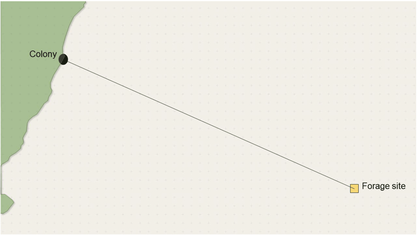
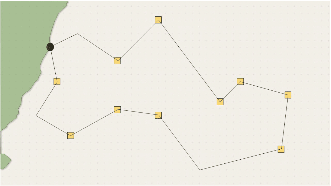
The modelled area within SeabORD is defined as a grid, with colonies and foraging sites assumed to be at the centre of the relevant grid cells. This is illustrated in the diagram below, with crosses used to indicate the centre of a grid cell. Currently, SeabORD uses a global grid at 30 arc-second intervals. SeabORD currently assumes birds undertake simple direct line flights (i.e. a great circle distance between two points on Earth).

Collision effects

If ORDs are included and lie in the direct path to be taken by a foraging bird, birds that are neither displaced nor barriered will follow the same initial flight path, and will be exposed to a collision risk for some for the route, shown below in red.

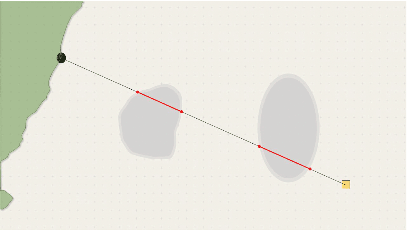
The distance covered within the ORD footprint is calculated by finding the coordinates where the flight line crosses the ORD polygon and calculating the great circle distance between those points. Birds are assumed to fly at a constant speed at all times, and the probability of death by collision is estimated for the time spent within the ORD. ORD-specific collision risks can be applied to the different ORDs encountered on the foraging route. Birds follow the same route 1-6 times per 'day', depending on forage availability and condition. Outward and return routes are identical.

Barrier and displacement effects

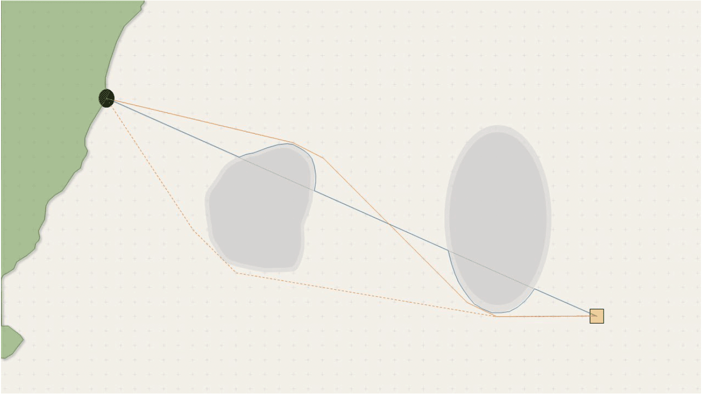
Birds that are categorised within SeabORD as barrier-susceptible or displacement-susceptible do not fly through an ORD. The user can select if the alternate route around the ORD is found using two alternative methods: the 'perimeter' method where barriered birds fly up to the edge of the ORD footprint/border region and then follow the perimeter until re-joining the direct line of flight between colony and foraging location (blue line, diagram below), or the 'A* shortest path' method where birds identify the shortest possible route between colony and foraging location whilst avoiding crossing into the ORD footprint/border area (orange lines, diagram below). The A* route may differ considerable from the direct line flight. This obstructed route-finding is done with all the obstructions known at the same time, so must be calculated for all required combinations of footprint, i.e., routes from A to B avoiding ORD 1 will be different if the bird has already re-routed around ORD 2. Outward and return routes are assumed to be the same.

Converting to use individual turbines

Adapting SeabORD to consider individual turbines requires the model to incorporate assumptions about three levels of avoidance – macro-avoidance where birds will act as currently modelled within SeabORD, avoiding the entire area of the ORD footprint and border area; meso-avoidance where birds will avoid an area immediately surrounding each individual turbine; and micro-avoidance where birds make last minute adjustments within the rotor-swept zone to avoid collisions with blades. Micro-avoidance is best handled within the collision component of the model, which is currently set up to use the sCRM. However, meso-avoidance will need to be included within SeabORD directly, in terms of adjusting birds' behaviour to avoid the immediate vicinity of turbines.

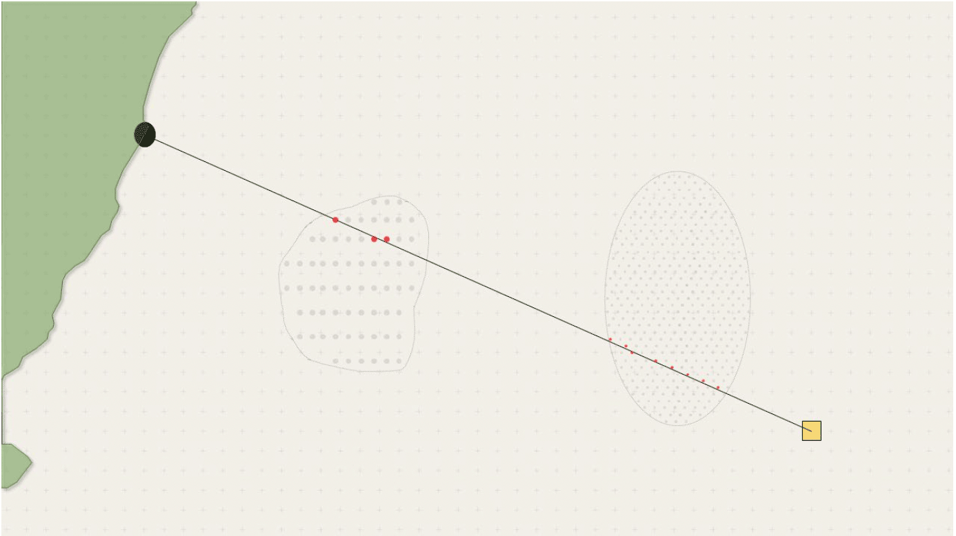
Within SeabORD, individual turbines could be defined as a point location with polygons around it denoting the collision risk zone (in which micro-avoidance will occur), and the meso-avoidance zone where it is assumed that displacement and barrier susceptible birds will not enter. An illustrative diagram for how this implementation might work within SeabORD is provided below – ORDs are now defined by an overall footprint polygon (for implementing macro-avoidance), and smaller turbine-polygons for defining areas of meso- and micro-avoidance.

Adapting SeabORD to work with individual turbine polygons in this way would not require much additional work to adapt collision risk probabilities – as is currently done for whole footprints, the model would calculate the amount of time spent crossing through the collision-risk zone, and use to this implement a probability of collision calculation which would determine if the bird suffers mortality. However, it would not be possible to use the same collision probabilities that are currently used, taken directly from the sCRM, because the collision probability would need to only include micro-avoidance within the rotor-swept area, with meso- and macro-avoidance being dealt with elsewhere in SeabORD's framework via the current displacement and barrier mechanisms. It would also be necessary to develop algorithms for how collision risk should be estimated for birds commuting through footprints, versus those foraging within footprints, and how to apportion foraging flight time in relation to turbine collision zones. For instance, if a bird chooses to spend 30 minutes foraging within an ORD footprint, we would need an algorithm for estimating the proportion of these 30 minutes in which the bird is potentially at risk in the collision-risk zones around nearby individual turbines.

In terms of technical implementation, SeabORD v1.5 (Matlab) requires each ORD polygon to be uploaded to the tool as a separate shapefile, and the user interface is restricted to five input files. If we were to allow for large numbers of polygons to represent individual turbines this would have to be amended, but is a minor change. SeabORD v2.0 (R software, under development in the MS Cumulative Effects Framework project) will allow for multiple polygons per shapefile, so will be set up to accept a polygon per turbine if required.

In terms of route-finding methods for simulating flightpaths to foraging locations, the most suitable current method is the 'A*' method. The 'A* shortest route' routines operate on the same spatial grid as the rest of the model. It uses an 'obstruction grid' defined as cells that are not accessible, which within the current version of SeabORD would be any cell that contains a turbine polygon. This will be problematic because currently grid cells are much larger than the collision-risk zone, or meso-avoidance zone that may be required for individual turbines. Therefore, depending on the turbine spacing, the grid alignment and orientation to the colony, the A* path may or may not be able to pass through the footprint due to the coarseness of the current grid. This means the current A* approach is unlikely to work for individual turbines. It might be possible to use a finer grid for just the obstruction map for the path-finding routine, leaving the main SeabORD grid as it is now. This would in theory allow for the birds to find a safe route between turbines but would be extremely slow.

More realistic flight lines and foraging tracks

The implementation of more realistic foraging tracks is discussed in more detail in Section 37, so here we limit our discussion to the more technical side of their implementation within SeabORD. The simplest solution to including more realistic foraging trips with multiple foraging locations and heterogeneous interspersed flight sections would be to predefine a large number of foraging tracks (as a set of coordinate pairs) and store them in a look-up table for the model to use during simulations (see example below). Birds would then randomly select a flight path from the stored list. This would be relatively straightforward to implement within SeabORD.

Model development would have to be undertaken to refine the foraging behaviour of birds within simulated trips, particularly in relation to the optimisation of the overall number of foraging trips per day, and the optimisation of the foraging time at different locations within a foraging trip in relation to prey availability and intake rate and energy gain. This is all achievable within SeabORD, but would require the development of new optimisation algorithms.

Outputs

SeabORD output can be in the form of graphs or csv data files. Currently, output can be provided per simulated time step over a season (e.g. changes for individual birds or chicks), per matched pair of runs (e.g. difference between baseline and scenario), overall season summaries, and overall summaries over multiple matched pairs of runs across different prey availabilities. Because birds within each simulation are fully tracked (i.e., the model records where they are and what they are doing within each time step), output could be modified to be more relevant to individual turbines or sets of turbines (footprints), with moderate adjustment to the model code, although this finer resolution output would have to be balanced against increased processing time required to record and save more detailed outputs.

Recommendations and key knowledge gaps

In order to implement bird behaviour around individual turbines it will be necessary to be able to parameterise different scales of avoidance behaviour – micro, meso and macros – such that biologically appropriate displacement and barrier behaviours can be simulated within SeabORD. Empirical evidence on these alternative scales of avoidance are currently only available for a limited number of species (e.g., gannets) and locations. Further empirical work is needed to better quantify these rates for different species, and to understand how rates may vary in relation to environmental and site-specific characteristics.

Recommendation 36. The quantification of uncertainty in displacement models must be achieved.

The objectives of this section are:

a. To summarise the current approach to quantification of uncertainty and variability within SeabORD, and outline the key limitations of this;

b. To assess the potential ways of improving the representation of uncertainty and variability within SeabORD, and to evaluate the feasibility of each;

c. To recommend specific steps that could be taken to improve the representation of uncertainty and variability.

Sources of uncertainty and variability within SeabORD

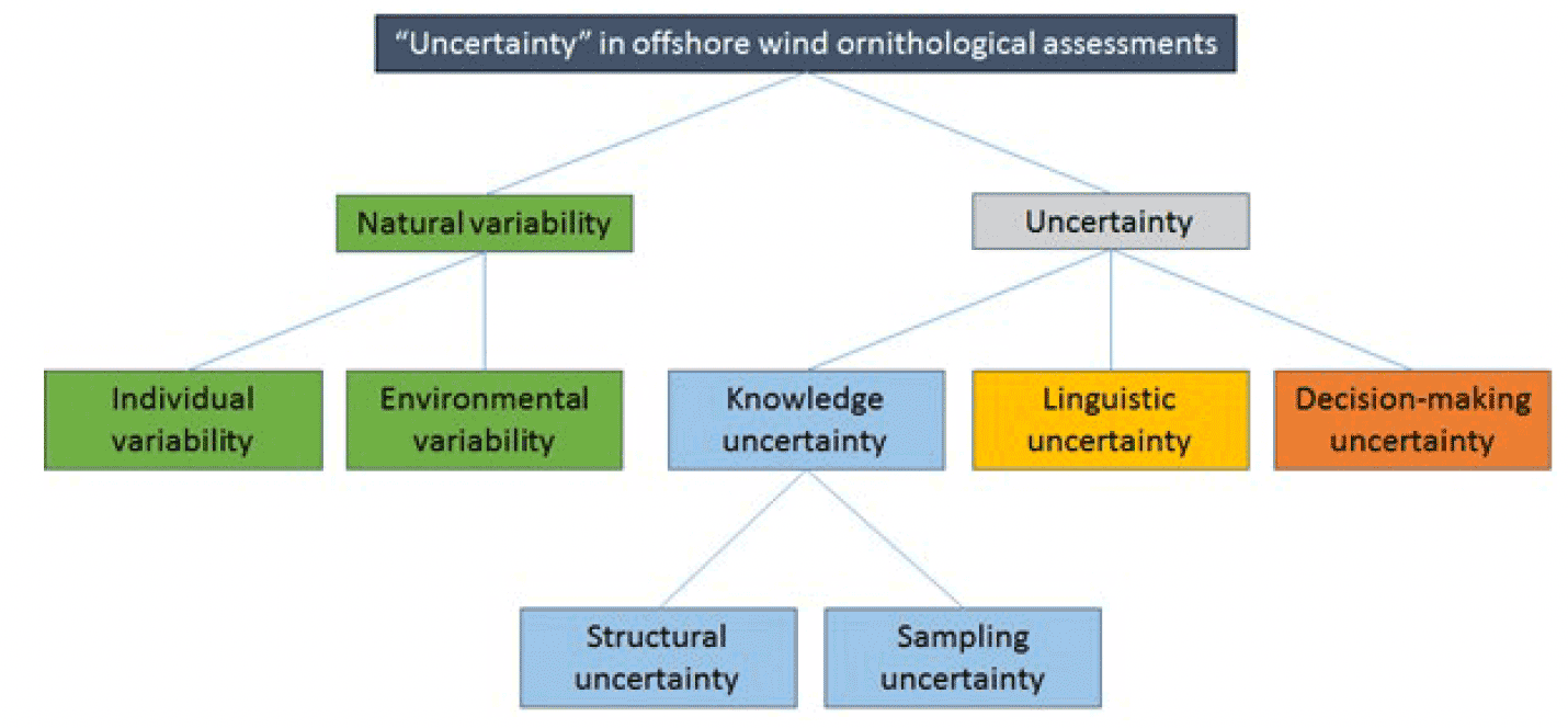
To improve the quantification of uncertainty and variability within a model such as SeabORD it is first necessary to identify the various types and sources of uncertainty and variation associated with it. Masden et al. (2015) characterized and summarized the key forms of uncertainty within offshore wind ornithological assessments (Figure 1), and the same forms of uncertainty are relevant when focusing on the individual component of the assessment – annual displacement risk during the chick-rearing period – that SeabORD is designed to address.

Variation and uncertainty are conceptually different to each other, even though they are often represented in similar mathematical and statistical ways. Variation is an inherent property of the system being modelled – so, in the case of SeabORD, a property of seabird behaviour, energetics, demography and response to offshore renewables developments. Importantly, because variation is a property of the system, it cannot be reduced by data collection or further analyses of existing data. It can, however, be characterised and quantified through data collection or through analysis of existing data. Estimated levels of variation may then be used within models of ecological processes, such as SeabORD.

Uncertainty, in contrast, is a function of how well we are able to understand, measure and represent an ecological process using a model. It arises from the fact that we only have partial, limited information about the system being modelled, and hence have an imperfect ability to describe the ecological process of interest. Increasing or improving data collection can lead to reduced uncertainty, as can the use of existing or new data to improve understanding of behaviour and processes through analysis or modelling. This form of uncertainty has been termed 'knowledge uncertainty' (Masden et al. 2015). Within ornithological offshore wind assessments, this knowledge uncertainty captures uncertainty that arises from our ability to understand and represent all of the ecological processes through which seabirds interact with offshore wind developments (ORDs). Within ornithological ORD assessments, uncertainty also arises through linguistic and decision-making processes. Linguistic uncertainty arises because language is vague and/or the precise meaning of words changes over time or between disciplines (Masden et al. 2015). Decision-making uncertainty relates to how knowledge and predictions are interpreted, communicated and used in the management and policy arena (Masden et al. 2014). Whilst important, these two additional sources of uncertainty are not considered further here, as the improved characterisation of these does not directly relate to the focus of this project, which is upon assessing the feasibility of improvements or extensions to SeabORD.

Knowledge uncertainty is driven by two key elements. The first is the mismatch between the assumptions that the model makes in describing ecological processes, and the way that the processes actually function - this is termed 'structural uncertainty', "model inadequacy", or, sometimes, 'process uncertainty'. The second is our ability to obtain data that adequately captures the states and processes underpinning interactions – Masden et al. (2015) term this 'sampling uncertainty'. Within a mechanistic model such as SeabORD this can be further divided down into uncertainty in the inputs (e.g. bird density maps, prey distribution maps), and uncertainty in the parameters (e.g. strength of the mass-survival relationship, assimilation efficiency).

We focus in this chapter on the potential to improve the representation of both variability and knowledge uncertainty (structural uncertainty, parameter uncertainty and input uncertainty) within SeabORD.

Current approach to estimating or assigning values of inputs & parameters within SeabORD

SeabORD contains two spatial inputs, and a relatively large number of model parameters (Table 1). The spatial inputs are maps of the distribution of prey (the "prey map") and colony-specific maps of the distribution of birds (the "bird density map"). The bird density maps are used within SeabORD to determine the trajectories of individual foraging trips. The potential for improvements to the representation of the spatial distribution of prey are considered in the previous section, and improvements to the representation of the spatial behaviour of birds, including both overall spatial distributions and the spatial dynamics of movements within an individual foraging trip, are considered in the later relevant section.

The values of most of the model parameters are currently assigned based on published literature or expert judgement (Table 1). However, there are three parameters that cannot readily be assigned in this way, and which are suspected to be important: the total amount of prey, a parameter that relates the intake rate to the time spent foraging (capturing the effect of prey depletion), and a parameter that relates the intake rate to the density of birds (capturing the effect of intra-specific competition).

The first of these parameters is calibrated against adult mass change and chick survival, and the latter two parameters are calibrated against the mean number of foraging trips made per day, and the mean and range of time spent foraging per day for each species. The latter calibration is only performed once for each species, and the calibrated values are then assumed to hold for all populations of that species. The former calibration, in contrast, is assumed to be population specific, and re-run whenever SeabORD is used on a new population – that is because the data used for the calibration (chick survival, adult mass change) are, at least in some cases, available for specific populations, and because it is biologically unrealistic to assume that the parameter being calibrated (total prey) is identical for all populations. Both calibration steps are currently relatively ad hoc – i.e. involve the users running SeabORD repeatedly until an acceptable level of fit to the observed data is achieved.

Table 19: Summary of the spatial inputs and parameters within SeabORD calculations, what type of value needs to be provided, units, whether the values vary between populations and/or footprints, and the source ("Lit" = from published literature; "EJ" = from expert judgement "EE" = from Expert Elicitation).

	What is provided?	Units	Varies between region, population &/or footprint?	Source
Spatial inputs
Bird density map	Map	Raster	Population	Modelling of GPS tracking data
Prey distribution map	Map	Raster	Region	Either linked to bird density map or assumed homogeneous
Model parameters
Total prey	Fixed value	na	Region	Calibration then Monte Carlo simulation
Baseline adult mortality rate		Proportion	Population	EE
Hourly collision probability*		Probability	Footprint	sCRM
Displacement susceptibility		Percentage	Region	SNCB guidance
Initial adult daily energy expenditure	Mean & standard deviation	kJ	No	Lit / EE
Initial adult body mass		Grams		Lit / EE
Initial chick body mass		Grams		Lit / EE
Critical mass below which adult assumed dead	Fixed value	Proportion of mean mass Grams		Lit / EE
Critical mass below which adult abandons chick				Lit / EE
Critical mass below which chick is dead		Grams		Lit / EE
Critical time threshold for unattendance at nest		Hours		Lit / EE
Number of time steps per season		Count		Lit / EE
Chick energy requirement		kJ/day		Lit / EE
Maximum prey intake rate		g/minute		Lit / EE
Intake rate parameters (2 parameters)				Calibration
Speed in flight		m/s		Lit / EE
Assimilation efficiency		Proportion		Lit / EE
Energy gained from prey		kJ/gram		Lit / EE
Energy cost of (a) nesting at colony, (b) flight, (c) resting at sea, (d) foraging and (e) warming food		kJ/day		Lit / EE
Maximum chick mass gain per day		Grams		Lit / EE
Energy density of bird tissue		TBA		Lit / EE
Survival metrics parameter				Lit / EE
Number of hours per time step		Count		Lit / EE

Current approach to quantification of variability in SeabORD

SeabORD is a stochastic, dynamic, individual-based, model that already incorporates a range of different sources of variability (Table 2):

a) inter-individual variability in the initial values of adult body mass, chick body mass and daily energy requirements at the start of the chick breeding season

b) inter-individual variability in displacement susceptibility – some individuals are simulated to be susceptible to displacement and/or barrier effects, whilst others are not, but this susceptibility is assumed to be constant over time (so any particular individual is either always susceptible to displacement or not susceptible to displacement)

c) temporal and inter-individual variability in the choice of foraging location – each individual is assumed to choose a foraging location at each time step

d) temporal and inter-individual variability in the choice of alternative foraging location if an individual is displaced by the ORD – if an individual cannot forage within the ORD footprint, because it is displacement-susceptible, it is simulated to choose an alternative foraging location from within an appropriate buffer region

Table 20: Summary of whether uncertainty and/or variability are accounted for each of the inputs to the main SeabORD calculations

	Uncertainty accounted for?	Variability between individuals accounted for?	Variability between timesteps accounted for?
Models inputs
Bird density map	No	Yes	Yes
Prey map	No	No	No
Model parameters
Total prey	Yes	No	No
Displacement susceptibility	No	Yes	No
Collision probability*	No	Yes	Yes
Initial adult daily energy expenditure	No	Yes	No
Initial adult body mass	No	Yes	No
Initial chick body mass	No	Yes	No
Critical mass below which adult assumed dead	No	No	No
Critical mass below which adult abandons chick	No	No	No
Critical mass below which chick is dead	No	No	No
Critical time threshold for unattendance at nest	No	No	No
Length of chick rearing period	No	No	No
Chick energy requirement	No	No	No
Maximum prey intake rate	No	No	No
Intake rate parameters (2 parameters)	No	No	No
Speed in flight	No	No	No
Assimilation efficiency	No	No	No
Energy gained from prey	No	No	No
Energy cost of (a) nesting at colony, (b) flight, (c) resting at sea, (d) foraging and (e) warming food	No	No	No
Maximum chick mass gain per day	No	No	No
Energy density of bird tissue	No	No	No
Survival metrics parameter	No	No	No
Number of hours per time step	Not relevant – internal model parameter

A technical summary of the way in which variability is incorporated into SeabORD for each of these is given in Table 3. Temporal and inter-individual variability in time budgets is also, at least to some extent, incorporated indirect, because time budgets are assumed, within SeabORD, to be linked to the choice of foraging location (since the foraging location is assumed to determine the total time spent flying, and the number of foraging trips per time step).

Table 21: Summary of how variability is accounted for within SeabORD, for each input /parameter that does incorporate or relate to variability

Input or parameter	Associated simulated quantity within model
	Name	Type of value	Which level?	How simulated from input/parameter?
Bird density map	Foraging location	Location	Time step within individual	Randomly, with probability of particular grid cell being selected proportional to the bird density value for that grid cell
	Alternative foraging location if displaced	Location		Randomly, with probability of particular grid cell within the "outer buffer" region (user-defined) being selected proportional to the bird density value for that grid cell
Displacement susceptibility (percentage of population)	Displacement susceptibility (for each individual)	Binary (yes/no)	Individual	Independent Bernoulli simulations
Hourly collision probability	Mortality from collision event	Binary (yes/no)	time step within individual
Critical mass below which adult assumed dead	Mortality from low mass during chick rearing period	Binary (yes/no)	time step within individual
Baseline mortality rate	Over-winter mortality	Binary (yes/no)	Individual
Strength of mass-survival relationship
Initial adult daily energy expenditure	Initial adult daily energy expenditure	Positive value	Individual	Independent simulations from a normal distribution with mean & SD
Initial adult body mass	Initial adult body mass
Initial chick body mass	Initial chick body mass

These sources of variability mean that there is variability in the final mass of individual birds at the end of the chick rearing period, and variation in whether or not their chicks fail. There is also assumed to be stochastic variation in the actual outcomes for each adult bird – e.g. final mass is assumed to be related (via a logit-linear model) to the probability of over-winter survival, but there is still stochastic variation in whether any individual bird actually survives or not. If SeabORD is coupled with the sCRM there is also variability in whether each individual dies from collision at each time step or not, with the sCRM and simulated daily time budget determining the probability of collision for each bird at each time step.

There are many other parameters for which temporal and inter-individual variability is not considered (Table 2), largely due to a lack of available information on the level of variability that might plausibly be expected.

Current approach to quantification of uncertainty in SeabORD

Whilst SeabORD accounts for a range of different sources of variability, it is currently much more limited in the way that it accounts for uncertainty. Variations between runs of SeabORD therefore arise in large part from stochastic variation in the set of individuals simulated, with this source of variation being largest when the populations being simulated are small. There is, however, one source of uncertainty that is currently explicitly accounted for within SeabORD – the total level of prey – and this is accounted for through a simulation-based (Monte Carlo) approach. The current advice to users is to run SeabORD multiple times (a relatively small number of runs, 10, being the standard choice, due to the model being computationally intensive to run), with a different level of total prey being used for each run. The range of total prey values to consider is determined through an initial calibration step in which an uncertainty range is specified for the percent adult mass loss over the course of the chick rearing period, and total prey values are selected so as to calibrate with the lower and upper ends of this range, whilst also ensuring that chick survival rates remain consistent with observed values. Total prey values are then simulated from within this range via stratified random sampling.

Relevant ongoing work

Within the MSS CEF project^[2] two important improvements to SeabORD are currently being made:

a) re-coding the model into R, whilst simultaneously attempting to reduce the computational time needed to run the model; and

b) automating the process of calibrating the level of total prey so that this does not require manual intervention from users.

The former development is an important step in improving the quantification of uncertainty within SeabORD, as most methodologies for defensibly quantifying uncertainty rely upon able to generate relatively large numbers of simulations from the model, and this depends, in turn, upon being able to run the model sufficiently quickly for this to be feasible.

Automation of the calibration process is also an important step in improved quantification of uncertainty, for two reasons. The first is that the current, manual, calibration procedure relies upon fairly extensive human intervention, which would make it infeasible to run SeabORD large numbers of times even if the computational burden of running SeabORD could be substantially reduced. The second is that methodologies for improving the quantification of uncertainty within the calibration step rely upon the calibration being based on a clearly defined and automatable algorithm, and so cannot be used until the current ad hoc approach to calibration has been replaced with a more algorithmic approach.

The key challenge in automating the calibration of total prey lies in the fact that only a very narrow range of total prey values lead to biologically plausible outcomes – most values of the total prey parameter are either associated with all birds dying, or all birds surviving, and this creates problems for standard calibration approaches. To overcome this issue we are developing a two-stage approach within the CEF project – the first stage involves using a simple deterministic model to determine a plausible range of total prey levels, and the second stage involves using SeabORD to calibrate within this range using standard numerical optimisation approaches.

Potential improvements: direct information on uncertainty in model inputs

• Still to be added: updated assessment of whether information in the literature exists to quantify variability (e.g. standard deviations) or uncertainty (e.g. standard errors) for any of the parameters for which this is not currently done.

The mass-survival relationship is a key component of SeabORD, and recent work (Daunt et al., 2020) has allowed uncertainty in this to be properly quantified; this is discussed further in the later relevant section.

Additional data collection

• Still to be added: identification of parameters for which data collection is the best solution – e.g. total prey

Expert elicitation

There are many situations in which the literature and available data are contradictory or inconclusive regarding the value of an input parameter and/or the uncertainty associated with this, and situations in which both sources of information are entirely absent. In many such situations, however, experts will have knowledge regarding both the value of the parameter, and the level of uncertainty associated with this, that go beyond anything that can be derived directly from either literature review or data analysis. In these situations, expert elicitation provides a mechanism for encapsulating this knowledge. Expert elicitation is, in essence, a formal process of representing expert judgement in a quantitative way, and it typically involves assessing judgements on the level and form of uncertainty alongside judgement on the true value of the input parameters (O'Hagan, 2019). Elicitation exercises typically involve multiple experts, in order that the judgements they incorporate relate to a community of experts, rather than to a single individual.

Running an effective expert elicitation exercise is challenging and time consuming. There are various pitfalls, and an extensive literature highlights the potential pitfalls in elicitation exercises, and outlines strategies and guidance for avoiding these (EFSA, 2014; Peel et al., 2018). A key issue in elicitation is the need to ensure that the different experts are all making comparable assessments – i.e. answering the same question. For quantities such as the SeabORD input parameters this is a crucial and difficult step, since many of these quantities are difficult to define in a way that is entirely precise and hence free from ambiguity, and some parameters can only meaningfully be interpreted within the context of a specific model for behaviour (e.g. the adult-chick prioritisation score). Expert elicitation exercises, consequently, often begin with a structured discussion in which the experts attempt to reach consensus on the interpretation of question(s) (O'Hagan, 2019), and this is likely to be essential for any elicitation of SeabORD parameters.

Another key challenge in elicitation lies in the quantification of uncertainty and/or variability. There are two key challenges in doing this. The first is that not all measures of uncertainty/variability are in a form that is likely to be possible for experts to meaningfully assess. It is known, for example, that standard deviations and standard errors are challenging to assess, as are extreme quantiles, and known that a poor choice of metric for encapsulating uncertainty can lead to systematic bias within the elicitation of uncertainty (). Quartiles and, especially, tertiles, in contrast, are quantities that (if explained in appropriate ways) can more naturally encapsulate the sorts of expert knowledge of uncertainty that are typically available, and thereby minimize such biases (Garthwaite et al., 2005).

The second key challenge is in distinguishing between variability and uncertainty. This relates to the choice of question: if we wish to assess the mean number of hours per day spent foraging, for example, then we could either consider the mean number of hours over time, for one birds, or the mean number of hours over time, averaged across all birds within a population. Both quantities would plausibly have the same "best estimate", but the levels of uncertainty in them would be very different, and would reflect different things – uncertainty in the former incorporates variability between individuals, in addition to uncertainty in the population-level mean, whereas uncertainty in the latter only incorporates uncertainty in the population-level mean. In situations where there is extensive variation between individuals (as is almost always the case for seabird species) the difference between these can be very large, which means that a precise formulation of, and understanding of, the problem being based is crucial in order for the elicitation to provide meaningful assessments of levels of uncertainty.

Alternative approaches to calibration

In Section 3.1 we have considered the potential for directly improving the quantification of uncertainty within the input parameters, through literature review, additional data collection or expert elicitation. If all input parameters could be defensibly quantified in this way, and there were no structural uncertainties within the model (i.e. the model assumptions corresponded entirely with reality), then these approaches would be sufficient for fully quantifying uncertainty in model outputs. In practice, models typically contain input parameters for which direct information is sparse or completely absent. This is certainly true in the case of SeabORD, and it is unlikely that the uncertainties in all of these parameters could defensibly be quantified. The values of those input parameters that cannot be directly estimated can instead be estimated by calibrating the model against observed data on model outputs, and the uncertainties associated with this process of calibration can be quantified. This calibration can also allow structural uncertainties to be identified and quantified – structural uncertainties arise if the model systematically deviates from reality even with an optimal choice of input parameters, as will commonly be the case when working with models of complex ecological systems.

SeabORD already performs some calibration of parameters – e.g. to determine two of the parameters controlling intake rate, and to estimate the total level of prey – but these are currently implemented in a relatively ad hoc way, and no attempt is made to quantify the uncertainty associated with calibration.

Optimisation-based approaches

Standard automated approaches to calibration often involve using optimisation algorithms to select the values of one or more input parameters that minimise the differences between observed and modelled values of key model outputs. A range of metrics are available to summarize the magnitudes of differences between modelled outputs and observed data, including sums of squares, sums of absolute differences or model likelihoods, and the optimisation can then be achieved using standard numerical optimisation algorithms. The simplest algorithms simply involve searching across a regular grid of possible input values for the set of input values that minimize the discrepancy metric. Grid-based search algorithms can be computationally slow, however, especially if the number of input parameters being considered is fairly large, so, in practice, alternative, more computationally efficient, approaches are usually used – e.g. gradient descent methods, which iteratively select the set of input parameters to consider by following the direction, within the space of input parameters, for which the values of the discrepancy metric change most rapidly. Optimisation algorithms usually require initial (starting) values to be specified, and use convergence criteria to assess whether the algorithms have indeed found the set of parameter values that minimise the discrepancy metric.

A key problem with optimisation-based approaches is that they are typically only able to find local maxima, rather than global maxima – this is problematic if there are many sets of input parameters that have roughly equal discrepancy from the observed data. This issue can typically be dealt with by restricting the calibration to focus only the set of parameters that can realistically be estimated by calibration against the available empirical data on model outputs – for SeabORD, for example, it is unrealistic to expect that the available output data could realistically be used to calibrate every single parameter of the model, so it will be probably only ever be feasible to calibrate a relatively small number of parameters using model output.

The other key problem with optimisation-based approaches is that they typically often little potential for quantifying uncertainty. Approaches based upon minimizing sums of squares offer a straightforward way of identifying the "best" set of input parameter values, for example, but do not automatically provide a framework for identifying other sets of parameter values that are compatible with the empirical data on the model outputs. Approaches they involve maximising the likelihood function (or, in practice, minimizing the negative log-likelihood) do allow quantification of uncertainty, as the negative of the hessian matrix of the log-likelihood, evaluated at the maximum likelihood estimate, can be used to approximate the covariance matrix of the maximum likelihood estimator (Azzalini, 1996). However, there is no obvious way of formulating the likelihood for a complex, simulation-based stochastic model such as SeabORD (unless using emulation, see Section 4.2.4).

Likelihood-free inference, ABC and GLUE

"Likelihood-free inference" refers to a broad class of statistical methods for estimating the parameters of stochastic models that can easily be simulated from, but for which a likelihood cannot readily be calculated, and for quantifying the uncertainty associated with this estimation process. As such, likelihood-free inference methods are a potential approach to use in calibrating a model like SeabORD. Unlike optimisation-based approaches, the likelihood-free inference approaches are explicitly probabilistic, and hence explicitly designed to quantify the uncertainty associated with calibration.

A widely used class of likelihood-free inference methods are Approximate Bayesian Computation (ABC) methods. ABC methods are conceptually straightforward; the simplest version of ABC involves:

a) defining a discrepancy metric that can be used to compare a summary statistic (or set of summary statistics) of the model output against equivalent summary statistic(s) for the observed data;

b) repeatedly simulating sets of input parameters from a prior distribution;

c) for each simulated set of input parameters generating a simulation from the model, and calculating the discrepancy between the summaries of this simulation and the summaries of the actual data;

d) accepting a set of input parameters if the discrepancy is equal to zero, and rejecting it otherwise.

This approach is called "Approximate Bayesian Computation" because, if the summary statistics are chosen appropriately, the sets of input parameters that are accepted by this algorithm are simulations from the posterior distribution of the parameters – i.e. they are equi-probable sets of parameter values, given the observed data, with a Bayesian framework. As with all Bayesian methods, this approach requires prior distributions for the input parameters to be specified: these can either be chosen to be informative (if judgement can be used to constrain the plausible values for these parameters) or diffuse (if there is little prior information on the values of the parameters). The key difference between ABC and standard Bayesian methods is that standard Bayesian methods require the likelihood of the model to be known, whereas ABC does not, and ABC can therefore be used for complex stochastic simulation-based models (such as SeabORD) for which standard Bayesian methods could not be used.

This very simple version of ABC provides a conceptually neat way of understanding how ABC works, but is of no practical use, except in the context of extremely simple models and data types. A key problem is that, in practice, it is very unlikely that a simulated dataset will ever be generated for which the discrepancy metric is equal to zero – i.e. for which the summary statistics of the simulated data exactly match of those of the real data. The easiest solution is to use the very simple version of ABC, but to accept all parameter sets for which the discrepancy is less than some small threshold, rather than only accepting parameters sets for which it is zero (e.g. Pritchard et al., 1999, Beaumont et al., 2002). By using a threshold greater than zero the method becomes an approximate, rather than exact, Bayesian approach, and this is one reason for the "A" ("Approximate") in the name. Even this version of ABC can be very computationally slow to use, however, especially if the prior distributions are diffuse (i.e. fairly uninformative). A key strand of literature on ABC has involved the development of faster algorithms, typically by embedding the ABC algorithm within another algorithm that is already relatively computationally efficient – e.g. ABC-MCMC (Marjoram et al., 2004) and ABC-SMC (Sisson et al., 2007). These algorithms can now be implemented within software such as Python (e.g. Klinger et al., 2018) and R (e.g. Jabot et al., 2013).

The "approximate" part of ABC also arises because, in practice, it is not always straightforward to choose appropriate summary statistics. For simple models and data it can be possible to identify the summary statistics to consider via theoretical arguments – ABC ideally uses "sufficient statistics" (statistics that, together, capture all of the information contained within the data that are relevant to the model), and for simple models, and data structures, these can be derived mathematically. However, for realistically complicated models – which certainly includes SeabORD - this is not possible, and in that case the idea is to select summary statistics that capture, in a more intuitive and less formal sense, the key features of the data that can be used for calibration of the input parameters. In this case, the summary statistics selected are unlikely to be sufficient statistics, which means that ABC is only, even with a threshold of zero for the level of discrepancy between data and simulations, an approximation to a Bayesian approach (hence the "A" within ABC). Statistical methods to try and identify the most appropriate set of summary statistics to consider have been developed (Fearnhead & Prangle, 2012; Burr & Skurikhin, 2013).

ABC algorithms are usually regarded as providing an approximate form of Bayesian inference, but they can also be viewed rather differently, as a way of accounting for structural error in the formulation of the model (Wilkinson, 2013).

ABC methods are related (Nott et al., 2012; Sadegh & Vrugt, 2013) to a widely-used methodology for quantifying uncertainty in hydrological models: "GLUE" (Generalized Likelihood Uncertainty Estimation; Beven & Binley, 1992; Mirzaei et al., 2015). As with ABC methods, the key practical drawback of applying GLUE methods to a model such as SeabORD, is that, despite attempts to improve computational efficiency by combining the GLUE approach with modern algorithms for efficiently exploring the parameter space (e.g. MCMC, Blasone et al., 2008), they rely upon the ability to generate relatively large numbers of model runs.

Emulation

The key issue with applying likelihood-free inference, ABC or GLUE approaches to SeabORD is that these approaches are designed for models that are fast to simulate from, and typically assume, and require, that the model can be run for a large number of sets of input parameter values. In particular, the practically useful implementations of these approaches, such as the ABC-MCMC and ABC-SMC algorithms, rely on being able to generate thousands, or tens or hundreds of thousands, of model runs, and the computational effort required to run SeabORD means that this is unlikely to be realistic within the foreseeable future.

An alternative area of statistical methodology, in contrast, is emulation, which is explicitly designed for models that are highly computer intensive and hence can only be run on a relatively small number of sites. Emulation involves approximating the mechanistic model (in this case SeabORD) using a relatively simple statistical model (O'Hagan, 2006; Gu, et al , 2018), which can have orders of magnitude lower computational expense. The statistical model can then be used to quantify the uncertainty associated with the estimated input parameter values, whilst accounting for the uncertainty that arises from the relatively small number of runs of the mechanistic model. Extensions of the emulation methodology can also be used to quantify, and account for, the presence of structural error in the model, also known as model discrepancy (Adrianakis et al 2015).

The central idea of emulation is to (a) run the mechanistic model (e.g. SeabORD) for a relatively small number of sets of input parameters, and (b) to fit a statistical model that describes how the key outputs of the mechanistic model vary in relation to the values of the input parameters.

One very simple form of emulation assumes that the model output can be approximated by linear combinations of the input parameters – i.e. by applying a multiple linear regression (MLR) to the mechanistic model outputs, where the input parameters are the covariates in the regression (Montgomery et al., 2012). Whilst simple, this approach is not very flexible, because it assumes that the relationship between input parameters and output variables within the mechanistic model has a relatively simple linear form. However, the reason that mechanistic models are used in the first place is because they capture complexities that are missed by such simple statistical models. Thus it is undesirable to make such strong assumptions when constructing the emulator.

An alternative to using a MLR formulation is a Gaussian process (GP, Rasmussen & Williams, 2006). A GP is a probability model for a random vector that is similar to a MLR in that there is an assumption of multivariate normality and the mean structure is usually a linear combination of covariates, namely, the mechanistic model input parameters in the case of emulation. However, the fundamental difference between a MLR and a GP lies in the covariance matrix, namely, how model outputs for different combinations of model inputs, the components of the random vector, are co-related. The correlation between model outputs in a MLR have nothing to do with the model inputs, while in a GP the correlation is a function of model inputs. With a GP, if a pair of input parameters are close together (have similar values), then the corresponding pair of model outputs will be close together with high probability. This covariance structure then captures what has been referred to as model smoothness, a small change in a model input parameter vector should not lead to some large change in the model output. Another distinction between a MLR and a GP is that a GP that emulates a deterministic mechanistic model (there is no stochasticity), which has been calibrated (using maximum likelihood or Bayesian inference) to a set of mechanistic model parameter inputs and model outputs is an exact interpolator: when those particular model parameter inputs are plugged into the GP, the predicted GP outputs will exactly equal the mechanistic model outputs. MLRs will almost never do that and what is happening is that the emulator's covariance structure is "mopping up" all the variation in the model output that the mean structure (the linear model) does not account for. We also note that there are alternative strand of emulation methods that do not require an assumption of multivariate normality but make broadly similar assumptions (e.g. regarding smoothness) about the mean and the covariance structures: "Bayes Linear" methods (Goldstein & Wooff, 2007).

Emulation methods capture the uncertainty in the mechanistic model outputs that arises from the fact that only a limited number of mechanistic model runs are available, and so can be used even in situations where only very limited numbers of model runs are available. The simplest applications of emulation to mechanistic models are cases where one assumes that there is no structural uncertainty, the mechanistic model is describing reality and there is no "Model Discrepancy" (Andrianakis, et al 2015), and that the mechanistic model is deterministic (there is no "Ensemble Variability", Andrianakis, et al. 2015). Thus there is no uncertainty for sets of parameter values at which the model has been run. However, there is uncertainty about how close the emulator predictions will match mechanistic model outputs at untried input parameter combinations, what is called "Code Uncertainty" (Andrianakis, et al 2015). There is also a fourth kind of uncertainty when comparing mechanistic model or emulator outputs to observed data and that is so-called Observation Uncertainty (OU, Andrianakis et al 2015), due to sampling variation or field measurement errors.

For both mechanistic models and for emulators, there is almost always uncertainty about what values of the input parameters will yield outputs that most closely match reality. For deterministic mechanistic models, and for emulators, differences between model outputs and observed data will reflect model discrepancy (differences beween model output and reality) and observation uncertainty, and differences from emulators will also include code uncertainty. One approach to determining parameter values is calibration, finding the combination of parameter values that yield predictions that minimise some measure of prediction error (Kennedy & O'Hagan, 2001). Another approach is "history matching" (Craig et al. , 1997; Verson et al., 2014; Andrianakis et al., 2015; Williamson et al., 2013) that differences from calibration in the sense that only parameter values that produce outputs with some specified level of discrepancy from observed data are acceptable, in other words there is the possibility that no parameter combinations are suitable, in contrast to calibration that always yields some combination even if the resulting predicted values might high quite high prediction errors. History matching proceeds in an iterative manner successively reducing the allowable space for parameter values, i.e., successively shrinking the "plausible region" of parameter values, with the possibility that there may not be a plausible region---a useful outcome in the sense that is reveals that the model is unacceptably inadequate (Goldstein & Rougier, 2009; Andrianakis, et al 2015).

Emulation methods were originally designed for use with complex deterministic models, whereas SeabORD is stochastic. Emulation methods have also, however, been adapted to work with complex stochastic models, including IBMs (e.g. Oyebamijia et al., 2017).

Emulation methods can be implemented in a range of different ways, including via a range of different R packages (RobustGaSP, DiceKriging, tgp).

Note that development of an emulator for SeabORD is planned to take place within an ORJIP Carbone Trust funded project, due to start in Spring 2021: however, that emulator is designed to approximate SeabORD outputs in relation to the characteristics of footprints and populations, so that the emulator can be used to predict the displacement effects that SeabORD would produce for new populations and/or footprints. This differs from the emulator outlined here, which would approximate SeabORD outputs in relation to the internal parameters of SeabORD, and would be designed to quantify uncertainty within SeabORD runs for a particular population and footprint or combination of footprints.

Model refinements - reducing structural uncertainty

The methods of Section 4.2 in principle allow us to identify, and to some extent, quantify the effects of structural uncertainty – i.e. the increase in uncertainty that arises when model assumptions do not correspond to reality. These approaches rely on using empirical data on model outputs to ascertain the existence of structural uncertainties, and to quantify their magnitude. In order to reduce structural uncertainties, however, we need to understand the sources of these uncertainties.

In practice, seabird behaviour is extremely complicated, and consequently it is likely that none of the biological assumptions that underpin a model like SeabORD are likely to be entirely true. This does not necessarily matter, because: "since all models are wrong the scientist must be alert to what is importantly wrong. It is inappropriate to be concerned about mice when there are tigers abroad." (Box, 1976). Some model assumptions may be incorrect, but nonetheless lead to models that provide a very good approximation to reality, whereas other modelling assumptions may be incorrect in such a way, and to such an extent, that the models built upon them are essentially useless as a tool for understanding reality. There are three key elements in prioritising whether a particular assumption needs to be revised:

1. the biologically plausibility of the assumption;

2. the sensitivity of key model outputs to the failure of the assumption;

3. the availability of data or information that could be used to reformulate the assumption to be more realistic.

A key point to note is that it is common in ecology for it to be widely accepted that an assumption is biologically implausible, but for that assumption to nonetheless be used extensively in modelling. This is typically because, although the implausibility of the assumption in known, there is no clear understanding of how the assumption could be formulated differently – and, crucially, of how the alternative formulation could be parameterized. Improvements to the realism of model structure and assumptions are, consequently, closely tied with data collection - the introduction of additional realism, and hence complexity, into model structure is typically only worthwhile if data (or published literature) are available in order to be able to represent and parameterize this additional complexity.

There are many ways in which the structure of SeabORD could be refined to improve biological plausibility, but our judgement is that the key priorities for further development are those that have already been identified as priorities (Nature Scot Marine Bird Impact Assessment Guidance Workshop Report, February 2020):, and which are discussed elsewhere in this report:

• improved representation of flight paths, and of the estimated bird density maps that underpin these;
• improving representation of overall prey levels, and of spatial heterogeneity in prey
• improved representation of displacement, barrier and collision effects;
• improving representation of behaviour, energetics and ORD interactions outside the chick-rearing period;
• improving representation of the relationship between adult mass at the end of the chick rearing period and subsequent over-winter survival.

We regard these as high priorities for improving the structure of SeabORD in part because they all represent key components of the model, but also because, in each case, we can propose specific actions that can be pursued in order to make the biological assumptions of the model more realistic, by refining the way that data are used to inform the model structure and parameters. There are other components of the model that are potentially influential, and currently contain biological assumptions that are likely to be over-simplistic, but where it is difficult to see how the model could usefully be improved, given current data or additional data that could currently be collected – perhaps the most obvious one is the way in which adults allocate energy gained to their own needs versus those of their offspring. This is clearly an important component of SeabORD (as it affects the extent to which displacement and barrier effects translate into impacts on productivity versus survival, reflecting the life-history trade off in long-lived species), but for which is it difficult to collect empirical data.

A comprehensive sensitivity analysis of SeabORD is needed in order to determine the relative influence of the different parameters upon the key SeabORD outputs.

Conclusions

SeabORD, as a stochastic individual-based model, is already relatively sophisticated in the way that variability (over space and time, and between individuals) is accounted for, but uncertainty is currently dealt with in a very limited way that only focused on a single parameter (total prey) and ignores uncertainty in other parameters and inputs. There is therefore considerable potential for improvement and refinement in how SeabORD quantifies uncertainty.

The most obvious sources of uncertainty and variability in SeabORD are the uncertainty and variability in the spatial inputs (bird density maps and prey distribution maps) and the values of each of the parameters. The spatial distributions of both birds and prey are likely to be key sources of uncertainty, but methods for quantifying uncertainties in the spatial inputs are discussed elsewhere in this report. As the model has around twenty parameters these are potentially very large sources of uncertainty. There is no single approach that is likely to simultaneously improve the quantification of uncertainty, and reduce the levels of uncertainty, within all of these parameters, so a range of different approaches is likely to be required. The possible approaches for each parameter are:

1. using published values from the existing literature, or analyses of existing data – where this is feasible;

2. new data collection – where this is feasible;

3. expert elicitation – where there is sufficient existing knowledge that experts should be able to meaningfully specify information about the parameter;

4. calibration against data on model outputs.

Calibration can only realistically be used as an approach for estimating a relatively small subset of the total number of parameters, because there are only fairly limited data (e.g. on adult mass) that can be compared against SeabORD outputs. Calibration, should, therefore be reversed for use with the set of parameters for which the previous three approaches are least viable (i.e. where the first two approaches cannot be used, and where expert elicitation is unlikely to be defensible).

For those parameters for which updated literature review, novel analysis, or novel data collection are not feasible expert elicitation provides the best option.

The calibration step does not currently allow for uncertainty, but statistical methods to allow this do exist, and we have reviewed a range of these here. Emulation seems the most appropriate of the approaches considered, because this provides a flexible framework for quantifying the uncertainty associated with calibration – and, crucially, because this approach is designed to deal with computationally intensive models such as SeabORD, and to account for this within the quantification of uncertainty. Crucially, emulation methods could also begin to address the other main source of statistical uncertainty within SeabORD – structural uncertainty – by allowing the level and form of structural uncertainty to be quantified (e.g. via history matching). The emulator would need to account for the stochasticity of SeabORD. Development of the emulator would require a set of SeabORD runs, in which the parameters being calibrated are varied. Although development of an emulator for SeabORD is already planned to take place (ORJIP/Carbon Trust funded project due to commence in Spring 2021), this is being developed in a different context (to use SeabORD in predicting displacement mortality rates for new populations and footprints), and is distinct from the emulator development that we have discussed here (which is focused on the quantification of parameter and structural uncertainty).

We have focused in this chapter upon improvements to the way uncertainty and variability are represented within the model, but the outputs of SeabORD could also usefully be revised and expanded to include additional summaries relating to uncertainty/variability, thereby enabling stakeholders to incorporate these model readily in to decision making.

Recommendations and key knowledge gaps

A. The current Monte Carlo (i.e. simulation-based) approach to quantification of uncertainty within SeabORD should be retained, but this approach should be extended to incorporate uncertainty in a much wider range of parameters and inputs than those currently considered. The simulation-based approach allows these to be integrated in to SeabORD as they become available – and so, in particular, would provide a mechanism for incorporating the estimates of uncertainty that future work proposed in other sections of this report would produce, specifically regarding bird distributions and foraging tracks and mass-survival relationships. As uncertainty is accounted for more comprehensively within SeabORD the set of model outputs should also be updated and expanded to capture this.

B. Further improvements to the computational efficiency of SeabORD are necessary so that it is possible to increase the number of simulations used in running it, since the reliability and stability of results obtained using the Monte Carlo approach to uncertainty are directly related to the number of simulations used.

C. A sensitivity analysis should be used to identify the parameters and inputs to SeabORD that are most influential in determining variations in model outputs, and he set of key parameters whose values are best estimated via calibration against observed data relating to model outputs should be re-evaluated based upon the outcomes of this sensitivity analysis..

D. The calibration process should be adapted so as to incorporate uncertainty, including the quantification of structural uncertainty. Emulation, and associated history matching methods, currently (given the computational constraints on running SeabORD) provide the most promising methodological approach for achieving this.

E. An updated literature review, and an associated expert elicitation exercise, should be used to update the values of the remaining parameters, and to quantify levels of uncertainty and variability associated with each of them.

Recommendation 37. Use of more GPS tracking data to characterise foraging trips made by birds to use in SeabORD models.

Current approach in SeabORD

Simulation of foraging trips under baseline conditions

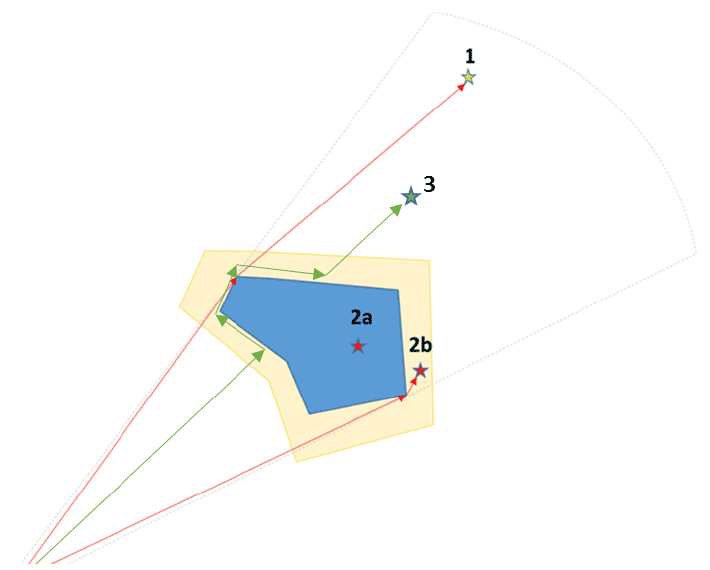
At each timestep for each individual, a foraging location (grid cell) is simulated with the bird density map providing the probability that each grid cell will be selected. Foraging locations are assumed to be independent between individuals and timesteps, and all trips within a particular timestep are assumed to be to the same foraging location. Individuals are assumed to fly from their breeding colony at a constant speed in a straight line to a pre-selected foraging location and return using the same route and speed to their breeding colony. The number of foraging trips per day is estimated using the range of number of trips from empirical data. Within this range, the number of trips is selected to minimize deficit between energy intake and energy requirements, and (if there is no deficit) to maximize nest attendance.

Simulation of foraging trips incorporating Offshore Renewable Development effects

Simulated foraging trips that incorporate Offshore Renewable Development (ORD) effects use baseline conditions with two considerations: barrier and displacement effects (Fig. 1).

Barrier-susceptible with pathfinding (1) If the bird selects a foraging location that lies beyond the ORD footprint (i.e. if a straight line from the breeding colony to the foraging location would pass through the footprint), and the individual is simulated to be susceptible to barrier effects, then the individual will retain the original choice of foraging location but will no longer take a straight line route from the breeding colony to this location. The individual will instead take a route that avoids passing over or through the footprint. The pathfinding option (A*) allows the individual to find the shortest route from the breeding colony to the foraging location that avoids passing through the footprint.

Barrier-susceptible with perimeter-following (3) The edge-following option means that the individual will attempt to fly in a straight line from the colony to the foraging location, until it encounters the boundary of the footprint. It will then follow the perimeter of the footprint boundary until it reaches the point where it can return to the original straight-line route.

The first version of SeabORD only included the perimeter option, but SeabORD was subsequently extended (Searle et al. 2018) to include the pathfinding option. The two options reflect different biological assumptions regarding the response of an individual to the footprint: the perimeter option assumes that the bird does not expect to encounter a footprint and so cannot select a route that avoids it until it reaches the perimeter of the footprint. The pathfinding option assumes that the bird has pre-selected the choice of foraging location and anticipates the presence of a footprint before leaving the colony so can choose the route to the foraging location that minimizes time and energy used (whilst still avoiding the footprint).

Displacement and barrier-susceptible (2a/2b) If an individual selects a foraging location within the footprint (Fig. 1; 2a), and that individual is simulated to be susceptible to displacement effects, it is assumed to select an alternative foraging location. The alternative foraging location (Fig. 1; 2b) is simulated from within a 5km buffer (Fig. 1; pale yellow polygon) around the footprint (Fig. 1; blue polygon), with the probability of any location (grid cell) being selected within the buffer as proportional to the distribution of bird density values within the buffer. The foraging trip from the breeding colony to the new foraging location is simulated in the same way as if the individual had originally chosen this as their foraging location (i.e. it is simulated to be a straight line unless the location lies within beyond the ORD footprint and the individual is assumed to be barrier-susceptible).

Seabird density map

The creation of a seabird density map is usually external to SeabORD unless the option is chosen to use a simple distance-decay function. In this case, a density map is created within SeabORD under the assumption that log(density) is proportional to distance from colony. In situations where GPS tracking data are available, the recommendation is that these data should be used to produce a density map which can be imported into SeabORD. A density map is defined as a raster file based on a regular spatial grid that quantifies the probability that an individual will select each cell on the grid as their foraging location.

SeabORD does not make any assumptions regarding the derivation of a density map but in applications of SeabORD to date, maps have typically been based upon modelling local GPS tracking data for the population(s) of interest using generalized additive models (GAMs). The current MSS CEF project (https://www.ceh.ac.uk/our-science/projects/cumulative-effects-framework) will enable SeabORD to also access the national colony-specific bird density maps produced by Wakefield et al. (2017), which fitted habitat association models to multi-colony GPS tracking data. Wakefield et al. (2017) maps have the advantage that they can be used for breeding colonies for which no local GPS tracking data are available. However, as they are based on extrapolating from the relatively small proportion of breeding colonies for which GPS tracking data were available up to 2017, they may be less defensible than maps derived from local GPS tracking data if the focus is on populations for which local GPS tracking data are available. GAMs have typically been used in applications of SeabORD to date because the focus of these applications upon the Forth-Tay region, on the east coast of Scotland, for which extensive local GPS tracking data are available for the key populations of interest (e.g. Forth Islands SPA, Fowlsheugh SPA and St Abbs Head to Fast Castle SPA).

Developing more realistic foraging trajectories

There are several improvements that could be made to simulate more realistic foraging trips (defined as a return trip from the colony to a foraging patch) within SeabORD. Assumptions made in the baseline simulations such as flying at constant speed and straight-line flight between breeding colony and foraging location do not generally reflect typical animal behaviour, which even when constrained by central-place foraging, tends to be complex and individualistic (Owen et al. 2019; Wakefield et al. 2015, Patrick et al. 2014). To develop more realistic foraging return trips, GPS tracking data are available for several key seabird species recognised to be susceptible to displacement and barrier effects (Peschko et al. 2020, Searle et al. 2018). Rather than flying directly from their breeding colony to a foraging location, tracking data show that birds exhibit many, different behaviours, at different locations, such as flying, resting on water, and foraging attempts. They return by different routes during a foraging trip (Chivers et al. 2012), and their flight speed varies depending on their activity and environmental conditions (Shamoun-Baranes et al. 2016). Time-activity budgets affect energy expenditure and so developing more realistic foraging return trips in SeabORD will aid the barrier and displacement simulations, which make assumptions around minimising energy expenditure.

For species with tracking data available, there are several approaches that could be used to develop more biologically realistic trajectories of foraging tracks. These range from typical movement models using step selection that characterise the behaviour of an individual animal through to models that characterise population-level space utilisation and habitat preference, which could be used to produce more realistic density maps. The approaches outlined below also set out statistical advances, which may help to overcome some of the limitations prevalent when analysing tracking data. Table 1 shows a summary of the current assumptions to model return foraging trips and density maps in SeabORD and the potential for improvements.

Table 22: Current assumptions used in SeabORD to simulate foraging return trips (or a density map*), and opportunities for improvement to develop more realistic foraging simulations (or a density map**) using tracking data.

Current assumption in SeabORD	Potential improvement in SeabORD
Straight-line return foraging trip	Accounting for non-straight line paths
One foraging location	Multiple foraging patches exploited
Constant speed of flying	Variable transit speeds, relating to activities
Spatial separation of behaviours limited to flying or foraging (foraging and resting at sea are assumed to occur at the same location)	Including more (species-specific) behaviours into track simulations
No uncertainty included	Measurement error accounted for
Ancillary data (e.g. explanatory covariates) not included	Ancillary data included
Density map created using distance decay function*	Density map created using track simulations**

The methods for potentially generating more biologically plausible trajectories and bird density maps can be divide into three main types - Hidden Markov Models, Continuous Time Hidden Markov Models and Habitat Preference Models - and we now outline the potential for using each of these methods within SeabORD.

Hidden Markov Models (HMMs)

Step selection function models are used to infer behaviour (e.g. foraging, resting at sea, diving) and estimate activity budgets of seabirds fitted with biologging devices. They can be used to investigate flight paths with respect to collision risk and displacement (Cleasby et al. 2015, Warwick-Evans et al. 2018, Peschko et al. 2020). A class of movement models that has become popular in ecology for analysing tracking data are Hidden Markov Models (HMMs), which are state-space models that assume the observed (state-dependent) time series is driven by an unobservable ('hidden') state process. The observed process is a function of latent (unobserved) states that describe the underlying behaviour of the individual and how this changes over time, described by a transition probability matrix (Morales et al. 2004). The observation process links the observed data to the hidden latent states, defined through a diagonal observation probability matrix. HMMs can account for serial dependence between observations (Patterson et al. 2008, Langrock et al. 2012), and are straightforward to implement aided by R packages such as moveHMM (Michelot et al. 2016) and momentuHMM (McClintock & Michelot, 2018). HMMs are implemented by assuming equally spaced (discrete) time intervals form a bivariate time series with step-length (l_t, distance between two locations), commonly parameterised as a gamma distribution, and turning angle (φ_t, angle between two locations), commonly parameterised as a von mises distribution, defining the changes between consecutive locations. Depending on the complexity of the behaviour states required, combining locational data with ancillary information such as accelerometer, time-depth recorders, or environmental covariates can achieve more plausible models. For example, where at-sea behaviour is required to be disaggregated into behaviour states beyond foraging and flying (e.g. resting on water, flapping flight, gliding flight, foraging, and taking off), accelerometer data can provide additional information to delineate these behaviours (Berlincourt et al. 2015).

However, discrete-time HMMs have limitations through both their assumptions and practical implementation. They do not typically consider measurement error in location but treat the state as part of a stochastic process (Patterson et al. 2008). Tracking data such as GPS observations are typically irregular in time as biologging tags are fitted to individuals and observations are transmitted to satellites when in range. They must usually be transformed into data with regular time-intervals as HMMs suffer from scale invariance, which makes it challenging to deal with missing observations (Patterson et al. 2017). Regularising tracks can introduce additional locational error that is not accounted for because discretisation makes assumptions such as individuals always move in a straight line between location fixes (straight-line interpolation), which is unlikely to be true. Finally, sub-sampling (known as data thinning) to regular time-intervals deals with autocorrelation but also discards locational information.

Continuous-time Hidden Markov Models (ctHMMs)

The limiting properties of discrete-time HMMs described above (straight-line movement assumption, regular time discretisation, sub-sampling, and ignoring measurement error) should ideally be accounted for to improve movement models with respect to more realistic trajectories and reducing uncertainty within SeabORD. A class of models that provides a promising avenue of methods development are continuous-time HMMs, which may help solve these issues. Continuous-time HMMs, as the name suggests, do not discretise time but extend HMMs to account for the state of the whole process (rather than just the previous observation as discrete-time HMMs do).

Integrated continuous-time Hidden Markov Models (ictHMMs)

Assuming that times and locations given (in the data) correspond to potential behavioural switches, integrated continuous-time Hidden Markov Models (ictHMMs) are a time-inhomogeneous version of a discrete-time HMM, defined at the potential switching times. However, behavioural switching is computationally expensive and so fast approximations can be implemented by limiting the number of switches in proportion to the interval between observations. The likelihood evaluation of ictHMMs can then integrate out the unobserved behavioural states, which ensures the approach is computationally efficient. Using a fully Bayesian approach, hidden states can be sampled using Forward-Filtering Backward-Sampling (Früwirth-Schnatter, 1994), which can be adapted for continuous-time models through uniformisation and allowing the model to be time-heterogeneous. This allows the location data to be irregular in time and does not require it to be regularised for the ictHMM to run. The efficiency of the approach allows for potentially many behaviours to be characterised (e.g. flying, foraging, resting, resting at sea) so that modelled behaviour more closely resembles the true behaviour of the species, allowing energetic budgets to be properly accounted for. Measurement error can be accounted for within this framework by including extra variables in the state of the Markov chain used for inference, which represent the true location at the time of each observation (Blackwell, 2019). By accounting for measurement error explicitly, a reduction in uncertainty can then be a possibility as this uncertainty can be propagated through the modelling framework of seabird tools for impact assessment. The lack of scale invariance of discrete-time HMMs places importance on the temporal scale chosen, which may not reflect appropriate scales for either the ecology of the species or the research question being investigated. However, ctHMMs have scale invariance and so are well placed to utilise available data as well as being less challenging for integration with other types of data.

Markov chain Monte Carlo continuous-time Hidden Markov Models (MCMC ctHMMs)

However, in general ctHMMs can suffer both from difficulty in implementation and a lack of parameter interpretability. Parton & Blackwell (2017) offer a solution to these issues through introducing a multistate movement model based on bearing and speed at time ≥ 0 (analogous to turning angle and step-length in discrete-time HMMs). The fully Bayesian approach utilises fine-scale sampling to reconstruct a more realistic path (than straight-line interpolation) between two observed locations using a Markov chain Monte Carlo algorithm (MCMC ctHMM). Using Gibbs sampling, behavioural switching rates are defined by a gamma distribution and the probabilities of switching (q) as the conjugate Dirichlet distribution. The movement process parameters are sampled on the conditional complete observation of both the reconstructed path and behavioural parameters and a Metropolis-Hastings algorithm is used with univariate Gaussian distributions (truncated below 0) to generate a random walk. To sample the path between two observations, it is broken down into smaller sections (sub-paths). This allows the path to be reconstructed into a more realistic trajectory as well as allowing for behavioural switching between observations. It is reasonable to conclude that there may be differences in activity budget results between ctHMMs and HMMs, as ctHMMs can switch behaviour states between observations whereas HMMs cannot. Switching behaviour states between observations seems not only credible but biologically extremely likely and so ctHMMs may offer additional insights (albeit with uncertainty) to reconstruct animal tracks in a more ecologically credible way. Uncertainty in the timings of behavioural switching can be visualised by sampling a large number of path reconstructions, which can then be used to estimate local space utilisation (see Langevin diffusion continuous-time model (LdctM) below). The results of this approach are also intuitive to interpret, describing aspects of movement of mean travelling speed and a propensity to the direction of movement, which are familiar concepts to users of HMMs. Like ictHMMs, this approach can also accommodate measurement errors. This can be done by including an additional parameter (assuming normally distributed independent errors) on the observation model.

The trade-offs for this approach are the choice of fine-scale temporal sampling which is used for sub-path length (i.e. computational cost is proportional to temporal resolution). However, high temporal sampling and so shorter sub-path lengths help the models to converge (Blackwell et al. 2016). Additionally, the number of bearing and speed parameters that require initial priors, which require 6 parameters for each behavioural state: If priors are too uninformative, this may cause problems with chain mixing and hence impact model run time and model convergence.

Continuous-time models therefore offer two potentially important solutions for important research questions relating to tracking data: (1) data integration of different data types (e.g. GPS and at-sea surveys) can be more readily combined because continuous-time models allow for scale invariance; and (2) seasonality can be incorporated into track simulations because ecological assumptions (e.g. central place foraging constraints) can be varied over time.

Habitat preference models

So far, step selection function models have been presented as approaches in which short-term insights are gained about the movement and behaviour of individuals using tracking data. However, population-level insights about long-term distribution and habitat preference are required for impact assessments, and more fundamentally, to understand the ecology of a species (Jones et al. 2015; Wakefield et al. 2017). Species distribution modelling using tracking information pools telemetry data from individuals and models the two-dimensional (latitude and longitude) as a utilisation distribution, which for central-place foraging species is their home range (Kie et al. 2010). This space use can be defined as 'the probability density function that gives the probability of funding an animal at a particular location' (Anderson, 1982). Since tracking data are presence-only, approaches such as use-availability (Aarts et al. 2008) and inhomogeneous Poisson process (Aarts et al. 2012; Fithian et al. 2013) are used to create locations where animals are (pseudo) absent to produce models of space use. Understanding changes in distribution is important in ecology and so habitat preference models that are predictive in time (e.g. into the future) and/or space can be developed to understand how and why animals respond to their environment (Wakefield et al. 2011; Raymond et al. 2015). From a modelling perspective, this is achieved through linking space use with underlying environmental conditions through Resource Selection Functions (RSFs; Boyce et al. 2002; Johnson et al. 2008). RSFs assess the probability that animals use a resource that is proportional to the availability of that resource. This accounts for heterogeneity in the environmental landscape that animals move through, which has differing availability depending on constraints (e.g. central-place foraging). Habitat preference is then the 'ratio of the use of a habitat over its availability' given that all habitats are available, which can be calculated through deviations in the direct proportionality between space use and (environmental) availability (Aarts et al. 2008).

The classes of models that have been discussed so far have commonality in their use of tracking data. Step selection models (discrete- and continuous-time) offer short-term behavioural insights about individuals whilst habitat preference models focus on long-term distributions at a population-level. However, when step selection models are scaled to population-level, they do not corroborate with habitat preference models as these models assume independence between telemetry observations (Michelot et al. 2019a). An advancement in SeabORD would be the option to derive utilisation distributions from simulated tracks, rather than relying on generating distributions using the decay function. This would be useful for species where tracking data are collected, but no species distribution maps are currently available (e.g. herring gull).

Langevin diffusion continuous-time model (LdctM)

One scalable solution is a Langevin diffusion continuous-time model (LdctM), which is a mechanistic movement model continuous in time and space (Michelot et al. 2019b). Position is modelled as a diffusion process with a gradient drift towards the limiting utilisation distribution. This is an extension of an MCMC step selection model for resampling tracking data to recover a utilisation distribution, accounting for autocorrelation between locations (Michelot et al. 2019a). The premise of these approaches is to think of movement models as short-term utilisation distributions, which as they are sampled more often, build towards a long-term distribution.

To summarise, the form of the LdctM is a continuous-time location process of an individual . A Langevin diffusion for the density (TT) is defined as a stochastic differential equation that includes Brownian motion where W_t is the multi-dimensional Brownian motion and is the gradient operator, under initial condition (X₀ = X₀) The utilisation distribution of the individual is linked to spatial (environmental) covariates using a standard parametric form of the Resource Selection Function. The movement of the individual is modelled in response to its environment and due to the diffusion gradient defined in the RSF, an animal tends to move towards better habitat (Michelot et al. 2019b). In practice, this approach can process tracks from multiple individuals simultaneously and include continuous explanatory covariates within the framework. Model selection can be carried out by comparing AIC of the joint model and model diagnostics include checking residuals for normality. An advantage of this approach is that the model is formulated in continuous time, negating the need to discretise either space or time, which often involves arbitrary choices that are not necessarily related to an appropriate ecological scale.

Recommendations and key knowledge gaps

Table 2 summaries the advantages and limitations of each method described in the preceding section, and how the method could contribute to more realistic simulated trajectories of return foraging trips (and density maps) through incorporating more biologically-realistic and statistically robust assumptions.

Table 23: Summary of the advantages and limitations of each methodology, and the possible contributions each method can make to more realistic simulated foraging return trips (and density maps*) in SeabORD.

Methodology	Advantages	Limitations	Contribution to more realistic trajectories
Hidden Markov Models (HMMs)	Account for serial autocorrelation through data thinning Can incorporate ancillary data into model Ease of implementation through accessible R packages	Treat measurement error in location as part of stochastic process so does not account for uncertainty Requires locations to be regularised time-steps Difficult to account for missing observations Not all data can be used due to autocorrelation Straight-line interpolation	Ancillary data included Multiple behavioural states
Integrated continuous-time HMMs (ictHMMs)	Handles irregular and missing observations (scale invariance) Integrate different data types	Difficulty in implementation and a lack of parameter interpretability	Measurement error included Can include seasonality in behaviour Ancillary data included Multiple behavioural states Variable transit speeds, relating to activities Including resting on the surface
Markov chain Monte Carlo step selection (MCMC ctHMM)	Handles irregular and missing observations (scale invariance) Straightforward interpretation of results More realistic trajectories Characterise behaviours between observations Measurement error can be incorporated	Requires 6 priors to be parameterised for each behavioural state Possible model convergence and issues with computational run time Environmental/ancillary data not yet incorporated into approach	Scale invariant Non straight-line interpolation More accurate activity budgets Multiple behavioural states Measurement error included Variable transit speeds, relating to activities Including resting on the surface Simulate individual tracks to form (local) utilisation distribution*
Langevin diffusion continuous-time model (LdctM)	Continuous modelling framework, which means that space and time do not need to be discretised. Handles irregular and missing observations (scale invariance) Explanatory covariates included Model selection and diagnostics well defined Model produces confidence intervals on parameter estimates Measurement error accounted for using a Kalman Filter	Difficultly in model fitting to real data, requires more testing	Scale invariant Simulate individual tracks to form (local) utilisation distribution* Ancillary data included Accommodate regions of attraction (e.g. foraging patches) Error propagated through model Variable transit speeds, relating to activities

Further uses of foraging trip simulations

In addition to the advances we have suggested above, simulating more realistic foraging trips based on tracking data could provide insight into more nuanced behaviours around ORD developments. For example, typical flight paths due to barrier effects could be incorporated into movement models using ancillary data. Barrier and displacement effects could be estimated empirically before, during, and after ORD construction, and non-permanent barrier effects such as varying spatio-temporal permeability could be identified empirically. We could use the approaches outlined above to generate simulations that make more biologically plausible assumptions about barrier and displacement effects, and then in future, once post-construction GPS tracking data are available, generate simulations that mirror the forms of displacement and barrier effects actually seen in these empirical data.

Recommendation 38. Expansion of SeabORD models to cover periods other than chick-rearing including non-breeding season.

During the non-breeding season, temperate seabird species tend to experience more unfavourable conditions than during breeding, associated with poor weather, reduced day length and lower food availability. At the same time, they are released from the constraints of central place foraging required for successful breeding and can therefore range more widely in search of areas with potentially more favourable conditions and experience less density-dependent competition. In light of this, potentially relevant parameters in the context of extending SeabORD would be at-sea locations/distribution, habitat association, time-activity budgets and body mass change. The concept of 'foraging trip' as defined during the breeding season is not applicable to the non-breeding season. Although some species (such as shags and herring gulls which are fully or partially resident and remain coastal year-round) attend their colonies in winter, colony attendance during this period is mainly relevant in the context of time-activity budgets.

To determine at-sea distribution and habitat association during the non-breeding season, two main types of data could be used: 1) data from tracking devices that remain on the birds year-round (mainly geolocators and in the case of large gulls, GPS loggers) and 2) data from at-sea surveys which however include records of birds from all age classes (i.e. not only adults). For kittiwake, puffin, guillemot, razorbill and shag, geolocation data are available from the Isle of May over multiple years. Additionally, a recent study by UKCEH of guillemots and razorbills has undertaken >400 geolocation deployments from 11 colonies across Scotland over three years. Similarly, a large multi-year dataset from Skomer and the Copeland Islands exists for Manx shearwaters (Gillies et al. 2020). Geolocation data on gannets have also been collected at several colonies (Bass Rock, Grassholm, Great Saltee; Deakin et al. 2019, Grecian et al. 2019). For the large gull species (herring and lesser black-backed gull) year-round GPS data are available from several colonies in the UK and the Netherlands (Shamoun-Baranes et al. 2017, Spelt et al. 2019, Thaxter et al. 2019, Van Donk et al. 2020). Overall sample sizes of tracked birds for each species are summarised in Table 24. Long-term at-sea survey data for all focal species are available from the ESAS database (Reid & Camphuysen 1998). Furthermore, species distribution models, including monthly predicted density maps, based on the ESAS data have been recently developed by Waggitt et al (2020).

Time-activity budgets could be established using data from geolocators that also record activity and temperature data (available for all focal species except large gulls) and from GPS and accelerometry data available for the two large gulls species. Assessing body mass change, however, would be extremely challenging since the birds spend most of their time at sea and, to our knowledge, mass measurements from the post-fledging and pre-laying phases are generally unavailable (see Task 1).

Table 24: Sample sizes of birds tracked over the non-breeding season for each study species (all colonies and years combined; data by colony are provided in the section on Task 1).

Species	N GLS	N GPS
Black-legged kittiwake	185	0
Common guillemot	384+	0
Razorbill	155+	0
Atlantic puffin	250+	0
European shag	444	0
Northern gannet	107+	0
Herring gull	0	ca.32
Lesser black-backed gull	0	<190
Manx shearwater	139+	0

Recommendations and key knowledge gaps

Given the increasing availability of non-breeding season data on distribution and activity, including of breeding individuals of known provenance, there is potential to develop an individual-based model for the non-breeding season. Such a model would simulate time/energy budgets and translate these into projections of adult survival and subsequent productivity, incorporating available data on non-breeding season distribution, activity, energetics and demography including carry-over effects on productivity. The model could be structured to apportion individuals to colony SPAs in species with sufficient data. The most logical species to focus on initially are common guillemot and razorbill, because of the availability of geolocation data from multiple colonies in the UK. Future studies could focus on expanding geolocation studies in other species, and to a larger suite of colonies. However, GPS tracking in the non-breeding season will remain a challenging goal for species not suited to harness deployments until leg-deployed GPS loggers are available at the appropriate size for the species in question. Significant knowledge gaps remain on the body mass and condition of birds outside the breeding season, and models would need to make assumptions of energy balance at different times of the year. As with geolocation data, some of the best data on body mass outside the breeding season is from guillemot and razorbill, further suggesting the importance to focus on these two species in the first instance. Further work is needed to determine if the best course of action would be to attempt to extend SeabORD to cover the non-breeding season, or if an alternative, simpler model structure might be needed due to the relatively lower data quality for bird movements and energetics during this time.

Recommendation 39. Uncertainty in mass-survival relationships to be incorporated into SeabORD.

Context

SeabORD (Searle et al., 2014; Searle et al., 2018) provides a mechanistic model of seabird behaviour, energetics, productivity and ORD interactions during the chick rearing period. The key mechanism through which displacement and barrier effects of offshore renewables are expected to impact on seabird populations is through their impacts on adult survival. Adult mortality through the chick rearing period is negligible, so displacement and barrier effects within the chick rearing period are primarily expected to impact adult survival through by reducing adult mass at the end of the chick rearing period, which, in turn, leads to reductions in over-winter adult survival.

The final component of SeabORD therefore involves translating final adult mass values of individual birds at the end of the chick rearing period into over-winter mortality of these birds. Although SeabORD is primarily a mechanistic model, the translation of adult mass at the end of the chick rearing period into over-winter mortality is modelled in a non-mechanistic way, by using statistical models to capture empirical relationships between mass and survival.

Current approach within SeabORD

The current version of SeabORD uses published relationships between adult mass at the end of the chick rearing period ("final adult mass") and annual survival rates, in order to convert simulated adult mass values into estimated over-winter survival rates. A technical description of how these relationships are used within the model is given in Appendix A. Note that annual survival rates and over-winter survival rates are effectively equivalent, given that there is negligible adult mortality during the breeding season for all of the species currently modelled by SeabORD. The same relationships are used to translate final adult mass into survival for baseline simulations and for simulations that have been generated in the presence of ORDs. This allows us to assess the impact of the ORD upon the adult survival rate by contrasting the paired model runs obtained with and without ORDs.

The conversion of simulated final adult mass values for individuals into an overall estimate of adult survival for each simulation run is currently based on previously published studies (Oro and Furness 2002, Erikstad et al. 2009). Both of these studies assume that survival is linked to mass through a logistic regression, such that

Survival probabilities are calculated separately for each individual, within both baseline and impacted runs, and an estimate of the excess mortality rate as a result of the ORDs is then obtained by comparing mean survival probabilities (averaged across individuals) between impacted and baseline runs of the model.

"Standardized" final adult mass is derived by calculating actual final mass, in grams, minus mean final mass under the baseline scenario, and, except for kittiwake, by then dividing this by the standard deviation of final adult mass under the baseline scenario (for kittiwake this final step is omitted).

The logistic regression model contains two unknown parameters, the intercept and slope. The intercept parameter is estimated using published data on annual mean baseline adult survival rates for the species (and, where available, population) of interest, and then taking the logit transformation of these rates, so that

The mean baseline survival values s₀ currently used are shown in Table 3-3 of Searle et al. (2018). These values were assumed to be appropriate for all of the Forth-Tay SPAs, and so have been used in all applications of SeabORD to date, but different rates would potentially be used if applying SeabORD to colonies in other regions for which local survival data are available (e.g. Shetland, Wales).

The slope parameter, which quantifies the strength of the relationship between mass and survival, is determined using values given in the published literature. For kittiwakes it is based on the value given in Oro & Furness (2002), and for all other species it is based on the value given in Erikstad et al. (2009). Published values do not exist for razorbill or guillemot, so we assume that they have the same value as that estimated for puffin in the Erikstad et al. (2009) paper. The estimated slopes are 1.03 (Erikstad et al., 2009) and 0.038 (Oro & Furness 2002). These values cannot be directly compared, however, because they relate to mass values that are expressed on direct scales: Erikstad et al. (2009) standardize mass so as to obtain a unit-free quantity, whereas Oro & Furness (2002) quantify the relationship in terms of absolute mass (in grams). This difference explains the reason that SeabORD standardizes mass differently for kittiwake than for the other species.

Issues with current approach

There are a number of issues with the current approach, and improvements to the mass-survival relationship were highlighted by SNCBs as one of the key priority areas for improvements to SeabORD (Nature Scot Marine Bird Impact Assessment Guidance Workshop Report, February 2020).

The first, crucial, issue is that the published mass-survival relationships currently used in SeabORD are based upon populations, and, for common guillemot and razorbill, species, that differ from those for which the model will be run. The black-legged kittiwake study was undertaken on a population in Shetland experiencing low food abundance, and the Atlantic puffin study was based on a population in northern Norway where the ecology of puffins including environmental conditions differs markedly from the UK. As such, both populations may have differed in terms of adult body mass and relationships between condition and survival from populations in the Forth/Tay region and in other regions that are of key interest for assessing impacts of ORDs. Furthermore, mass/survival relationships in common guillemots and razorbills may differ from Atlantic puffins.

A second key issue is that SeabORD does not currently account at all for the uncertainty in the mass-survival relationship. This is important because we might expect the form and strength of the mass-survival relationship to be a large and important source of uncertainty when using SeabORD to estimate ORD effects on adult survival.

A third key issue is that the published relationships used to quantity the mass-survival relationship are based upon data that characterise variations between individuals under baseline conditions (i.e. in the absence of an ORD). The use of these relationships within SeabORD assumes that the effects on survival of reductions in mass on individuals due to ORD displacement/barrier effects are comparable to the effects on survival of natural variations in mass that occur between individuals. This may not necessarily be a sound assumption, especially if mass is acting partly as a proxy for other traits that are linked to over-winter survival, rather than as a direct driver of over-winter survival.

Another, more technical, issue with the current approach is that the baseline mean survival rates simulated by SeabORD will, in general, differ somewhat from the baseline mean survival rates specified for s₀ (Appendix C), because of the nonlinearity of the logit function used in modelling the mass-survival relationship.

Potential solutions

A recent study (Daunt et al., 2020) used data from the Isle of May to produce empirical estimates of mass-survival relationships for four species: common guillemot, razorbill, Atlantic puffin and black-legged kittiwake. As part of long-term monitoring, adult birds are caught during the breeding season and individually marked, and a proportion are weighed. This protocol has been undertaken over multiple years in these four species, allowing the relationship between body mass and survival to be estimated. The quality of data varies among species. Puffin and kittiwake data have been collected across a wide range of dates during the breeding season, whereas guillemot and razorbill body mass data are focussed on a narrow window during chick-rearing. A further challenge with razorbills are small samples sizes of marked birds with mass data. Finally, puffin data that were most suitable for this analyses are older, collected over a period from the late 1970s to mid 1980s, since body mass was taken over a broad range of dates over several years during this period and not since. For the other three species, the data come from a long period up to the near-present. A sophisticated statistical modelling framework was used, which accounted for the effects of age and inter-annual variability (the model structure is described in Appendix C), and provided a full quantification of uncertainty.

Incorporating the estimated relationships from Daunt et al. (2020) into SeabORD, in place of the current mass-survival relationships, would overcome two of the key issues raised in the previous section: the fact that the current relationships are based on populations, and often species, that are not directly related to the populations and species to which SeabORD is being applied, and the fact that uncertainty in the mass-survival relationship is not currently accounted for.

At face value, use of the revised relationships from Daunt et al. (2020) within SeabORD seems rather daunting, as it requires knowledge of the pseudo-age structure of the population [the term pseudo-age, used in modelling by Daunt et al. (2020), is the number of years since a bird started to breed]. Given that the pseudo-age structure is dependent on breeding success in past years (the determinant of initial cohort sizes) and mortality in previous winters (the process by which initial cohort size becomes reduced), settlement rates (the fraction of birds of some true age which birds become breeders and hence take on a pseudo-age of 0), knowledge of pseudo-age structure seems unlikely to be accurately determined. However, if we regard the population average effect on survival within the models of Daunt et al. (2020) as contributing to the baseline mean survival, then we can avoid the need to consider the age structure (Appendix B). This allows the estimated slopes of the mass-survival relationships within Daunt et al. (2020) to be incorporated into SeabORD in the same way that the estimated slopes from Erikstad et al. (2009) and Oro & Furness (2002) are currently incorporated.

An additional point to be aware of is that for Atlantic puffins and black-legged kittiwakes, the Daunt et al (2018) model's combined year effect terms contains an effect of random year-to-year variation in mean colony level mass on survival. However, these effects were very weak and uncertain (For Atlantic puffins, this posterior mean was -0.0080 with standard deviation 0.0318, whilst the equivalent figures for black-legged kittiwake were 0.0058 and 0.110). In addition, we see little reason to suppose the relationship between the between-year mean mass and survival is likely to better approximate any ORD effect on survival than the relationship between survival and individual bird mass at the end of the breeding season. For these reasons we consider this additional point can reasonably be ignored.

There is always uncertainty in the value of the mass effect on survival. This could be overcome by repeating the calculations of individual-specific survival probabilities using different values of the slope parameter, in a manner akin to parametric bootstrapping with one value of the slope parameter, per bootstrap iteration, so that across iterations the values of the slop parameter used are representative of the posterior distribution of values calculated by Daunt et al. (2020). This aligns with the simulation-based approach already used by SeabORD to account for uncertainty in total prey levels, and with the potential ways of improving the representation of uncertainty within SeabORD.

Uncertainty in the mass-survival relationship is higher for some species than others (Daunt et al., 2020). It is only for Puffins that the 95% credible interval (the Bayesian equivalent of the 95% confidence interval) for the estimated mass-survival relationship does not contain zero. Thus, despite the advanced statistical analyses conducted in Daunt et al. (2020), considerable uncertainty remains about both the magnitude and even the direction of the relationship between body mass and survival. This is particularly the case for razorbills, where very little data was available, and in this case we recommend applying the new, revised relationships for puffins or guillemots. The choice between the species to use is complex, because razorbills show some ecological similarities with puffins (e.g. foraging behaviour, Dunn et al. 2019) and others with guillemots (timing of moult, winter distribution (Glew et al. 2018; 2019) but ultimately have a different ecology and life history from both species, so neither equation may be appropriate. until new data are collected that allow for a robust estimate of the relationship between mass and survival in razorbills, we propose that SeabORD should be refined to allow the mass-survival relationship for razorbill to be based on the relationships for both guillemot and puffin and an equal combination of the relationship for these two species. An equal combination is appropriate at this stage based on the ecology of razorbills and the other two species. In practice, this could be achieved by including a slider input to SeabORD, that allows the weight given to the two species to be varied (e.g. from 0%, 50% and 100% being based on puffin). Results for intermediate percentages would be based on combining the entire distribution of the parameters associated with the estimated relationships, not just the best estimates for these parameters, and so would include uncertainty – the Bayesian approach used in Daunt et al. (2020) renders this a natural approach.

Conclusions

It is technically possible, and relatively straightforward, to incorporate the revised mass-survival relationships from Daunt et al. (2020) into SeabORD, and to do so in a manner in which the mean survival probability across individuals is equal to the value specified for the scenario being considered (Appendix E). It is also possible to incorporate uncertainty in these relationships, through the use of a simulation-based approach that aligns naturally with the overall approach used to quantify uncertainty within SeabORD. The incorporation of uncertainty is key, because, in practice, assessments are designed to be precautionary, and hence need to consider the range of uncertainty associated with the estimated annual effect. Representing the range of uncertainty in effects on annual survival will, by including quantiles of estimated effects within SeabORD output, allow stakeholders to assess the plausible upper limit of values for estimated displacement effects.

There are substantial caveats with the current relationships used in SeabORD, and many of these would remain with the revised relationship. Most importantly, the estimated relationships between body mass and survival are derived from naturally-occurring between-individual variation in survival, not imposed differences driven by restrictions on access to feeding ground, and it is an untested but essentially unavoidable assumption that the associated estimates of the mass-survival relationships are applicable to estimate variation in survival due to ORD impacts. However, revising the relationship would resolve a number of key issues with the current way this is represented in SeabORD – crucially, by allowing species-specific empirical estimates of the relationship to be used, and basing these estimates on more relevant and up-to-date data and more realistic modelling than for the current relationships.

One caveat of both the existing and revised approach (the fact the simulated mean survival from SeabORD will not match the baseline mean survival value used to calibrate the model, because of the logit transformation) could be overcome through an iterative procedure (Appendix C).

The revised relationships are more defensible than the existing relationships due to three reasons: Firstly they are based on populations more geographically relevant to UK offshore renewables and thus likely have more similar behaviour than those considered in Oro & Furness 2002 and Erikstad et al. 2009; secondly, they are based on many more years of data than prior studies, which in some cases involve only one year of measurement; thirdly, they use a more sophisticated modelling methodology, incorporating for example age effects, uncertainty in body mass measurement and observation, and most importantly a rigorous consideration of year to year changes in survival probability unrelated to body mass.

Thus, we recommend use of the revised relationships contained within the posterior distribtions for in Daunt et al. (2020) for all species. In the case of razorbills, where we see substantial uncertainties due to a paucity of raw data, we would advise using a weighted average of parameter percentiles for Atlantic puffins and common guillemots from the newer study. Given current evidence on the ecology of three species, we recommend that the relationship for puffin, for guillemot and a relationship based on equal weighting of the two species

Recommendations and key knowledge gaps

We recommend replacing all current mass survival relationship estimates within SeabORD with the corresponding estimates from Daunt et al 2018, with the exception of Razorbills, which should use a composite estimate derived from Atlantic puffin and common guillemot estimates from the same report. We recommended that the uncertainties associated with the revised relationships should, alongside this, also be incorporated into SeabORD, via a simulated-based approach, and that the outputs of SeabORD should be revised to include additional metrics that characterise uncertainty.

We also recommend that new empirical studies are undertaken to improve data sets on mass of breeding adults during the course of the breeding season. Existing monitoring data, while useful, were not designed with this question in mind. New studies would aim to collect data over a broader range of dates during the breeding season, in particular later into chick-rearing, but would require careful planning to ensure that they can be done in a way that does not unduly disturb breeding adults and their young.