Seabird study data - best practice development: study
This study developed best practice guidance to combine seabird survey data collected from different platforms based on a literature review, expert knowledge and a bespoke model development including sensitivity analysis. This can be used in environmental assessments for planning and licensing.
3 The state-of-the-art in seabird distribution modelling
3.1 Overview of species distribution modelling
Statistical analyses of spatial survey data aim to address four questions (Aarts et al. 2008). 1) How many individuals there are within a survey area (abundance estimation), 2) Wherethey are in space (population distribution), 3) Why they are there (habitat associations), 4) Where else they might be, and where they might go if the environment changes (spatial extrapolation and forecasting).
A puritan taxonomy of SDMs
At first sight, the diversity of methods available for converting spatial data to prediction maps can seem overwhelming. However, there is an emerging hierarchy in the methodological literature that considerably simplifies our effort to outline recommendations for best practice. We can present this as a succession of four branchings, leading up to our recommended approach of inhomogeneous point process models (Figure 1).
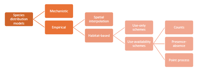
Spatial predictions can be generated by building mechanistic models of animal movement and demography from first principles and scaling them up to population distributions (Moorcroft et al. 1999, 2006, 2008, Moorcroft 2012). Arguably, models with a high biological detail (e.g. based on principles of physiological tolerance, movement behaviour and social interactions) bring greater insights and predictive capability (Kearney and Porter 2009, Hefley and Hooten 2016, Robinson et al. 2017). However, mechanistic modelling can be quite demanding technically and is generally more vulnerable to model misspecification and over-parameterisation. Misspecification will result in models that disagree with the data and over-parameterisation will generate models that cannot be sufficiently informed by the available data. For example, the series of papers by Moorcroft et al. cited above, which form the state-of-the-art in mechanistic distribution modelling, require specific assumptions about animal movement and rely on sufficiently mathematical users who can formulate and manipulate partial differential equation models. Alternatively, and more readily, the analysis can be done by mimicking observed patterns of space-use with the aid of empirical, statistical models (Guisan and Zimmermann 2000, Guisan and Thuiller 2005, Guisan et al. 2017). The deciding trade-off between mechanistic and empirical models is one of realism and predictive capacity against the ease of use and robustness to misspecification.
Within this class of empirical models (see review by Matthiopoulos and Aarts 2007), we can distinguish between models that merely reconstruct the spatial density of a population (such as kernel smoothing, additive smoothing, or geo-statistical methods) and regression methods that rely on habitat information as explanatory variables. Spatial density estimation methods rely on geographical proximity and the existence of spatial autocorrelation (Levin 1992) to interpolate between observation points and map density in unobserved space, or alternatively, to smooth a finite data set of synoptic observations into a population-level expectation of usage. Density estimation methods focus on removing spurious variability from the predictions, but aim to stay as close as possible to the observations. Therefore, their ability to describe the available data is often better than that of habitat models (Bahn and Mcgill 2007). Habitat models, on the other hand, are not by default spatial, since they are fitted in environmental (or niche) space (Pearman et al. 2008). Consequently, the greater ability of habitat models to interpolate and extrapolate spatially relies on the quality and relevance of their underpinning covariates. Nevertheless, the need to include such covariates when modelling seabird distributions is not in doubt (Camphuysen et al. 2004). The deciding trade-off between density estimation and habitat models is one of faithfulness to the particular distributional data collected and the ability to extend predictions beyond the spatial and temporal frame of data collection.
Within the class of habitat models, we distinguish between two main categories. The first, are known as profile methods and they argue that knowledge of where, in niche space, a species occurs is sufficient to understand its fundamental niche and map its current and future distribution. Broadly, this category includes methods such as climate envelope models and the use of multivariate statistical methods such as PCA (Robertson et al. 2001) for the analysis of presence only methods (reviewed in Pearce and Boyce 2006). The alternative class of use-availability schemes either contain representative information on the distribution of organisms (i.e. presence and absence), or they supplement presence data with availability data, allowing the models to contrast the habitat choices that organisms made, with the options that they had available to choose from. The broad area of use-availability schemes includes the vast literatures on resource selection functions (Boyce and McDonald 1999, Morris et al. 2016) and maximum entropy approaches (Elith et al. 2011, Merow et al. 2013). Profile methods have been critiqued extensively in the methodological literature (see Pearce and Boyce 2006 for a review), and there is really no sound scientific reason for choosing to use a profile method.
The final decision stage is mostly perceptual, relating to how space is conceptualised for the purposes of modelling the data. For example, space may be thought of as a regular grid (e.g. comprising squares, or other regular forms of tessellation, such as hexagons - see Grecian et al. 2016). In that case, the spatial data take the form of counts and are modelled by appropriate probability models such as the Poisson. Alternatively, space may be thought of as continuous and different spatial locations may be characterised by whether a species was present or absent. In that case, spatially reference data take the form of zeroes and ones and the most appropriate probability model is Bernoulli (Aarts et al. 2008). Yet another approach within the continuous space framework is to imagine that observations of organisms appear at random locations almost like pin-lights that blink in and out at different time frames of observation. This framework, known as the Inhomogeneous Point Process, models the occurrence of events within a unit of time and space as originating from a smooth intensity surface, describing the instantaneous and infinitesimal rate of the Poisson process (Chakraborty et al. 2011, Aarts et al. 2012, Fithian and Hastie 2013, Renner et al. 2015, Fletcher et al. 2019, Miller et al. 2019). It is an elegant approach that makes an implicit comparison between use and availability, captures heterogeneities in the distribution of the population (e.g. due to environmental covariates) but, can with equal ease, use the intensity surface to represent heterogeneities in the distribution of spatial observation effort (so that, regions that receive no observation effort will have a zero intensity when modelling the data). The deciding trade-off between count, presence-absence and point process models is in whether the user feels comfortable in conceptualising infinitesimal quantities and is happy to relinquish the notion of explicitly contrasting use and availability for the advantage of greater spatial and temporal precision in model fitting and prediction.
Hybridisation of SDMs
Different modelling approaches to species distributions are often presented as non-overlapping, much as we did in the preceding section. This often gives the impression that the only way to deal with multiplicity of approaches is to compare their performance and choose the best (e.g. Oppel et al. 2012). However, there is a methodological kinship between many of these approaches that is rarely apparent in the applied literature. Having so far organised the literature as a sequence of three strict dichotomies and a final trichotomy (Figure 1), it is good to take a less clear-cut, but more synthetic and conciliatory view on the above decisions. It is, in fact, the case that a hybrid approach is possible that retains the best elements of all the approaches discussed above.
Specifically, if one starts from a purely empirical model it is possible to move it towards a higher mechanistic content. In the simplest case, this can be done by carefully considering the biological relevance of the set of covariates that are offered to the model (Bell and Schlaepfer 2016). It is also possible to construct more sophisticated covariates using mechanistic models to try and increase the explanatory power of empirical models (Kearney and Porter 2009, Matthiopoulos et al. 2015). More recently, it is becoming possible to fit structurally complex models directly to data either by likelihood approaches, but most often, via Bayesian approaches. These developments have come mostly from the field of integrated population modelling (Matthiopoulos et al. 2014, Zipkin and Saunders 2018, Yen et al. 2019). As well as data-integration, the main benefit of integrated models is their capability to deal with non-linear features, a feature characterising most biologically realistic (i.e. mechanistic) models. We will use this aspect of hybridisation in this report when considering density-dependent effects on seabird distribution.
Also, the separation between spatial and habitat-based models can be made less strict. Geo-statistical models can accept habitat covariates and habitat models can accept spatial autocorrelation structures (Dormann et al. 2007). A considerable advantage of these models is that they optimally account for variability in the data (but see Hodges and Reich 2010). A perceived limitation of this approach is that predictions from hybrid spatial-habitat models are tied to the spatial extent of the data collection. We will discuss these issues at length later in the report and use them to construct spatial-habitat hybrid models.
The separation between use-only (or, profile) models and use-availability models is perhaps the most clear-cut of the branchings in Figure 1. Profile methods are problematic because, by ignoring the availability of different habitats, they interpret the habitat choices of organisms as purely the result of preference, not as a combination of preference and availability (Matthiopoulos 2003a). Profile models also misappropriate the ecological term "niche" because they aspire to define a species' viable hyper-volume in environmental space, and yet make no explicit connection between habitat data and population trends representing information on viability (Peterson et al. 2011, Matthiopoulos et al. 2015). Therefore, profile methods are fundamentally flawed from an ecological perspective. And yet, despite their limitations, their aspiration is worthwhile. Using habitat models to make sense of population viability should be a key objective in our search for defining critical habitat and in driving conservation efforts. Recent publications (Matthiopoulos et al. 2015, 2019) have shown how this can be achieved in practice by using the more defensible option of use-availability methods as a platform to build upon. We will briefly discuss how these methods could be used to integrate non-spatial data with spatial models.
Data types commonly used for SDMs are count, presence-absence and presence only (Hefley and Hooten 2016). Count data can be divided into point counts (e.g. point or line transects) and quadrat counts (comprehensive count in an area) (Hefley and Hooten 2016), although the distinctions between those two can be blurred. Presence-absence (or occupancy) data may either originate from count data that have been converted to binary form, or they may be the result of survey effort units that were terminated as soon as the species was detected once (Hefley and Hooten 2016). Finally, presence only data may include observations from known survey effort units (e.g. telemetry), or alternatively unknown effort surveys (such as museum records, or some citizen science programmes). Several papers (Warton et al. 2010, Aarts et al. 2012, Fithian and Hastie 2013, Hefley and Hooten 2016) have shown that the separation between count, presence absence and point process models is not substantial. Indeed, all of these methods can be thought of and re-formulated as inhomogeneous point processes. Furthermore, widely used spatial modelling packages such as MAXENT, can be thought of as point process models (Fithian and Hastie 2013, Renner and Warton 2013). Conversely, computational methods used for efficiently fitting point process models to data make use of spatial discretisation, similar to grid-based methods, but using more efficient schemes tailored to the data (Lindgren 2015).
During the rest of this report we will move towards recommending an approach that, while based on an empirical, habitat-driven point-process model, is capable of incorporating mechanistic (non-linear) features, using explicitly spatial information and is able to provide useful results for future assessments of population viability. Our approach will be based on the principles previously outlined by work funded by Marine Scotland (Oedekoven et al. 2012a, 2012b) and we will expand on these ideas, exploiting the opportunities offered by multiple surveys. Only around 7% of peer-reviewed marine SDM publications since 1992 have focused on seabirds, a total of 16 papers (Robinson et al. 2017). Although this survey excludes several publication-quality reports on seabird SDMs from the grey literature (Burt et al. 2009, Bradbury et al. 2011, Petersen and Nielsen 2011, Rexstad and Buckland 2012) it is nevertheless an indicator that we need to also look more broadly at the lessons learned from marine survey methods in general, as well as the transferrable elements of the ensuing analyses.
3.2 Overview of marine survey methods
Historically, and until the 1970s, knowledge of the distribution of seabirds around the UK comprised little more than maps of breeding colonies and the expectation that seabird numbers were probably high in the waters around them (Camphuysen et al. 2004). However, the need for risk assessment (and hence, more detailed spatial surveys of at-sea distribution) has been driven by the rapid developments in the energy industry (initially oil extraction, but then marine renewables and more recently, platform decommissioning). Initial efforts focusing on strip-transect designs (Tasker et al. 1984), were followed by stratification of distances from the observer (into detection bands) and by fully developed line-transect designs (Buckland et al. 2001, Thomas et al. 2010). Line transects have been undertaken by boat or aircraft and current best practice for survey design is summarised in (Camphuysen et al. 2004, Certain and Bretagnolle 2008, Oedekoven et al. 2012a, 2012b, Webb and Nehls 2019). Indeed, (Oedekoven et al. 2012b – based on earlier work by Camphuysen et al. 2004) give an excellent overview of the four distinct types of data collection in seabird research: boat surveys, visual aerial surveys, digital aerial surveys and vantage point surveys. More recent projects have also looked at tracking data to describe seabird-at-sea distributions – such as the RSPB FAME/STAR analysis and the Norwegian SEATRACK programme – both of which aim to describe seasonal spatial distribution patterns from tracking data sets, potentially even ignoring all of the other data types. We return briefly to tracking data in Section 7.5,
Line transect methodology has prompted the development of distance sampling methods (Buckland et al. 2008, Thomas et al. 2010) which deal with imperfections of the observation process such as decaying detectability of the subject with increasing distance from the observer (Buckland et al. 2001), the overall detectability at zero distance (Buckland et al. 2001) and the effect of environmental conditions on detectability (Marques and Buckland 2003). Although the original application of these methods was in estimating total population size, they have since been extensively applied to the estimation of relative abundance in order to create species distribution maps, often in response to habitat covariates (Clarke et al. 2003, Hedley and Buckland 2004, Oedekoven et al. 2012a, 2012b, Thiers et al. 2014, Waggitt et al. 2019).
| Source of bias |
Description |
Strip w. |
Baseline pr. |
|---|---|---|---|
| Distance effect |
Detection distance is the main variable in line transect analyses. |
✔ |
|
| Vantage height |
Determined either by the observation deck on a ship or the flight altitude of the aircraft. |
✔ |
|
| Study species morphology |
Smaller animals may be harder to see, and body pigmentation may camouflage them against background. |
✔ |
✔ |
| Behaviour of species |
Diving birds may be missed, and flocking birds may be over- or under-counted. |
✔ |
|
| Platform effects |
Smaller boats may be more vulnerable to movement resulting from wind or waves and noisy engines may conceivably repel animals. Conversely, animals that have developed vessel-following behaviours may be attracted by the presence of a boat. |
✔ |
✔ |
| Visibility conditions |
Weather and time of day will affect visibility. More generally, noise will be a problem for methods that use sound attenuation, although this is less important for seabirds. Conditions may change during a single survey or, even, a single transect, affecting the apparent abundance of the species. |
✔ |
✔ |
| Digitisation |
Although transfer of visual data to digital form is likely to be supervised by human technicians, processing of digital images may require some level of automation. This could result in over, or under-counting. |
✔ |
|
| Observer experience |
Different observers with different levels of skill or training may be introducing biases in their visual detections. These biases may remain consistent within observers, or they may diminish with experience. |
✔ |
✔ |
A simplistic but instructive statement about distance sampling is that it uses statistical modelling to bring line transect surveys closer to the original assumptions of strip transects. The effective detection distance derived from distance sampling methods allows us to assume that all event occurrences (i.e. birds) within an idealised strip of that width are detected with the same probability while all events outside that strip are missed. New field methods using digital photography from aerial platforms, yielding a relative density of birds per unit area, (Buckland et al. 2012, NaturalEngland 2019) are now the only survey method accepted by the regulator in some countries (e.g. Germany). These developments bring us full-circle to the strip transect as the gold standard. Therefore, counts that have been (or can be interpreted to have been) obtained from strip transects are the necessary starting point for analyses of population size and population distribution.
There are several aspects of the survey specification that can affect detectability but they all reduce to two main effects: the probability of detection at zero distance, and the effective detection distance from the observer. We use Table 1 to enumerate a variety of survey biases and illustrate that their effects can be entirely captured (i.e. corrected for) by modelling these two aspects of strip transects (even if this correction may, in some cases, require additional, calibrating data).
In this report, we, therefore, assume that the data correspond to strip transects, an assumption that would be correct for the raw data in the case of digital aerial surveys, but which implies a distance sampling pre-processing stage for line transect data (both ship-borne and aerial). Particularly in the setting of a multi-survey study (e.g. for the purposes of synthetic data generation in this project), a computational treatment of distinct surveys requires that each survey is concisely and uniquely characterised by a set of parameter values. In this report (see for example Section 3 of the accompanying vignette), the design specification of a survey is reduced to six characteristics. We divide those into characteristics of span and detectability. We outline them below, and also take the opportunity to collect all of the recommendations made by the pivotal report of (Camphuysen et al. 2004) for ship and aircraft survey design under each characteristic.
Span characteristics
Survey extent. Particularly with regard to marine developments, "it is recommended that a high resolution grid should be deployed, covering an area at least 6x the size of the proposed wind farm area, including at least 1-2 similar sized reference areas (same geographical, oceanographical characteristics), and preferably including nearby coastal waters (for nearshore wind farms only)" (Camphuysen et al. 2004). As we will discuss in the transferability section of this report (Section 5.5), it is important to conduct a cross-sectional sampling of space, but also to achieve as much spread of environmental conditions in the data, unaffected by expectations of where the species is likely to be.
Spacing of successive count locations. The spacing of locations will be determined by the combination of platform speed and sampling intervals. For ship surveys, "time intervals are recommended to be one or five minute intervals (range 1-10 m, longer time intervals are acceptable when less resolution of data is required; short intervals are preferred in small study areas), with mid-positions (Latitude, Longitude) to be recorded or calculated for each interval. Preferred ship's speed should be ten knots (range 5-15 knots)" (Camphuysen et al. 2004). For visual aerial surveys, "speed preferably 185 km h-1 at 80 m altitude. GPS positions should be recorded at least every 5 seconds (computer logs flight track)". Currently implemented digital aerial surveys are based on either still images recorded at intervals pre-determined to achieve a specific percentage coverage or continuous video recording, with image width set to achieve the target coverage.
Spacing between transects. Ship-based, "survey grid lines are recommended to be at least 0.5nmi apart, maximum 2nmi apart". Aerial "transects should be a minimum of 2 km apart to avoid double-counting whilst allowing the densest coverage feasible" (Camphuysen et al. 2004). Currently implemented surveys aim for distances of 2 km (ship), 2-3 km (aerial visual) and typically 2.5 km (aerial digital), although the latter varies depending on the target coverage percentage.
Transect orientation. Three main considerations enter the determination of the orientation of transects: statistical effort (e.g. avoiding overlaps), logistical constraints (e.g. need to avoid off-effort segments), geomorphological constraints (e.g. coastline and shallow water avoidance in ship surveys). No direct recommendations on this issue were provided specifically for seabirds by Camphuysen et al. (2004) but a general, concise discussion of automated transect design pertinent to this issue can be found in (Strindberg and Buckland 2004). Digital aerial methods, particularly those conducted farther offshore where variations in relation to distance to coast are expected to be reduced may also be oriented to minimise glare from the sea surface.
Detectability characteristics
Effective detection distance (strip width). Ship-based, "line-transect methodology is recommended with a strip width of 300 m maximum. Subdivision of survey bands is recommended to allow corrections for missed individuals at greater distances away from the observation platform. Preferred ship type is a motor vessel with forward viewing height possibilities at 10 m above sea level (range 5-25 m), not being a commercial or frequently active fishing vessel… Preferred ship-size: stable platform, at least 20 m total length, max. 100 m total length". In practice, current visual surveys use banding (ship bands 0-50,50-100,100-200,200-300, aerial visual bands are variable but often used are 44-163,163-282,282-426,426-1000. Note that unless 'bubble' windows are available 0-44 m is missed due to restricted view) and truncation distances (ship, 300 m one-sided survey, aerial visual 1 km two-sided) and aerial digital surveys use a strip width that will depend on flight height (300 m for still and 500 m for video). Other recommendations pertain to potential effects on the decay of detectability with distance. For example, it was suggested that, "the grid should be surveyed such that time of day is equally distributed over the entire area (changing start and end time over the area to fully comprehend effects of diurnal rhythms in the area)", also, to "use an inclinometer to measure declination from the horizon" and to avoid "observations in sea states above 3 (small waves with few whitecaps)" .
Baseline detection probability (detection at zero distance). Similar considerations relate to the baseline detection probability. For ship-based surveys, "no observations in sea state 5 or more to be used in data analysis for seabirds. Bird detection by naked eye as a default, except in areas with wintering divers Gaviidae. Scanning ahead with binoculars is necessary, for example to detect flushed divers. Two competent observers are required per observation platform equipped with rangefinders, GPS and data sheets; no immediate computerising of data during surveys to maximise attention on the actual detection, identification and recording. Observers should have adequate identification skills (i.e. all relevant scarce and common marine species well known, some knowledge of rarities, full understanding of plumages and moults). Observers must be trained by experienced offshore ornithologists under contrasting situations and in different seasons". Correspondingly, for visual aerial surveys, it is recommended using, "high-wing aircraft with excellent all-round visibility for observers. Two trained observers, one covering each side of the aircraft, with all observations recorded continuously on Dictaphone. No observations in sea states above three (small waves with few whitecaps)" (Camphuysen et al. 2004).
Survey particulars for exemplar species
In general, boat platforms are slower than aerial ones. Visual aerial surveys are fast but are characterised by lower detection rates than digital ones and fly lower so can cause flushing or avoidance in susceptible species. Digital aerial surveys are fast and fly higher, hence having lower risk of response behaviour and yield high rates of detection and species identification. Nevertheless, the relative accuracy of visual v digital methods in marine surveys is situation- and species-dependent (Furness 2016). More specifically, regarding the relationship of the four exemplar species to each of the three platforms: Gannets and great black-backed gulls are likely to be attracted to boats, kittiwakes probably not, whereas guillemots will avoid boats and be hard to spot (on the sea) as well as having a proportion of the birds underwater when the survey passed by. Visual detection from the air is likely to be good for gannet and great black-backed gulls but lower for guillemots. Species identification may be problematic for kittiwake, as a small gull species. Availability bias (birds underwater) may be particularly problematic for guillemots and sun glare may also be an issue for all of them. In digital aerial surveys, detection should be good for all four species although some kittiwakes may be classed as small gull species and great black-backed gulls as large gulls.
Contact
Email: ScotMER@gov.scot