Offshore wind energy - sectoral marine plan: seabird tagging feasibility
How to undertake a seabird tagging study for species and colonies potentially impacted by the sectoral marine plan for offshore wind energy
Sample size analysis
GPS
Methods
The ability to determine a species’ home range in relation to its breeding colony will be linked to both the number of birds which can be tracked, and the duration of any deployments. Several approaches have been developed in order to make inferences about the power of tracking datasets to quantify species home ranges (Beal et al., 2023; Soanes et al., 2013; Thaxter et al., 2017). We draw from the methods developed by Soanes et al. (2013) and (Thaxter et al. (2017) to make inferences about the benefits of prioritising a greater number of tag deployments (e.g. by using cheaper tags often with short term attachments) or longer term deployments (e.g. by using tags with solar panels to recharge batteries, which are often more expensive and require longer term attachment methods) in relation to defining a species home range.
We considered four datasets in this analysis (Table 4). There were discrepancies between datasets due to differences in the technology and methodologies used. Three of the studies used IgotU tags, which require recapture of the bird to download data, while the fourth used UvA tags, which allow remote download, meaning tags remain on individuals for a longer period of time, giving more trips per individual (Table 4). In contrast, whilst datasets from IgotU tags had fewer trips per individual, tags were deployed on a greater number of birds, helping to increase the sample size. We standardised methodology as much as possible to allow for a fair comparison of results between species. Following Soanes et al. (2013), and in contrast to Thaxter et al. (2017), we use trips as the basis of our analysis, rather than days, given the shorter deployments of the tags considered here. Consequently, for consistency, we use number of trips for all datasets. All data analysis and processing was done in R 4.2.0 (R Core Team, 2022), and the analytical process followed is set out in Figure 14.
| Species | Colony | Device | Year/years | Number of birds | Number of Fixes | Number of Trips | Fix Rate |
|---|---|---|---|---|---|---|---|
| Kittiwake | Whinnyfold | UvA | 2021 | 20 | 223172 | 1047 | 10 min/10 sec |
| Guillemot | Isle of May | IgotU | 2010, 2012, 2013, 2014 | 80 | 131807 | 241 | 2 min |
| Razorbill | Isle of May | IgotU | 2010, 2012, 2013, 2015 | 40 | 80309 | 192 | 2 min |
| Gannet | Bass Rock | IgotU | 2015, 2016, 2018 | 50 | 457707 | 535 | 2 min |

Data processing
To identify trips, and exclude tracks restricted to movements around the colony, we defined a 1000m buffer around the centre of the tagging location. Drawing from previous analyses, sequential trips were identified when an individual left and re-entered this buffer (Figure 14). Only complete trips, where birds re-entered this buffer were included in the subsequent analysis. Once trips were assigned, datasets were examined for erroneous positions and trips by visual assessment of plots, and any erroneous positions were removed.
Analysis
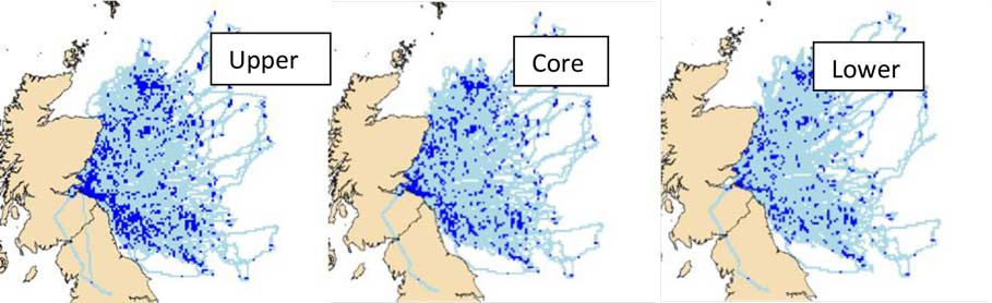
Given that we needed to use an iterative sampling of a number of birds for a number of set trips, each bird has to have the same number of trips, to control for bias in results by individual bird behaviour (Soanes et al., 2013; Thaxter et al., 2017). We followed Thaxter et al. (2017) by defining an initial sample size for each dataset, employing a core sample (median birds, median trips), alongside a lower sample (fewer birds, more trips) and an upper sample (more birds, fewer trips) (Figure 14). All initially defined sample sizes can be found in Table 5.
| Species | Colony | Sample | No birds | No trips |
|---|---|---|---|---|
| Kittiwake | Whinnyfold | Upper | 20 | 26 |
| Kittiwake | Whinnyfold | Core | 18 | 30 |
| Kittiwake | Whinnyfold | Lower | 16 | 35 |
| Gannet | Bass Rock | Upper | 51 | 3 |
| Gannet | Bass Rock | Core | 37 | 6 |
| Gannet | Bass Rock | Lower | 27 | 9 |
| Razorbill | Isle of May | Upper | 36 | 3 |
| Razorbill | Isle of May | Core | 29 | 4 |
| Razorbill | Isle of May | Lower | 26 | 5 |
| Guillemot | Isle of May | Upper | 64 | 3 |
| Guillemot | Isle of May | Core | 49 | 4 |
| Guillemot | Isle of May | Lower | 26 | 5 |
Using a bootstrapping approach, we investigated the relationship between cumulatively increasing number of birds or trips and area used (km2). For each bootstrap iteration, the algorithm selected a sample of birds providing the desired number of trips needed. The algorithm then sequentially added birds to the sample to yield a matrix of time spent in each 2 km2 square each day, and then cumulatively summed the time for each square across days. We then ordered squares by the summed time spent in them (from greatest to least) such that the minimum number of squares needed to produce the desired occupancy levels could be calculated. We repeated this process for all birds sequentially added to the bootstrap for the given starting sample. For a desired sample of birds, occasionally more individuals were available than the number required because birds sometimes had the same duration of data available; in those instances, the algorithm randomly selected the desired number of birds from all those with available data. Because of computing time and the number of samples investigated, we limited analysis of each dataset to 1,000 bootstraps (Bogdanova et al., 2014). We used non-linear modelling to fit relationships between area use and the cumulative number of birds in each bootstrap. As with Thaxter et al., (2017) we considered six candidate models, with the most parsimonious for each bootstrap selected using Akaike’s Information Criterion (AIC). Models where ∆AIC </= 2 were considered to be competitive. Using the best-fitting bird-area curve for each bootstrap, we estimated the area use of the populations together with the back-transformed number of birds needed to describe 95% estimated area use of the population (Soanes et al., 2013).
For respective populations, data for colony size was obtained using the Seabird Monitoring Programme database. For Bass Rock, we used the closest estimate which was from 2014. For the different species at Isle of May where multiple years of data were used, we took the average colony size during the years in which data was collected. For all combinations of increasing numbers of days and birds, we fitted curves. Box-and-whisker analysis was then used to assess the variance of back-transformed predictions of the number of birds needed (Borger et al., 2006). Where the number of birds included in the starting sample fell within or exceeded the interquartile range of the predicted number of birds, that number was interpreted as a minimum sufficient sample size to characterize area usage.
Results
Kittiwake
Data were collected from 20 GPS tagged birds at Whinnyfold in 2021. Tags remained attached to birds for 18 – 47 days, collecting data on 26 – 91 trips (Figure 15). The data were then used to create starting grids for the upper, core and lower starting samples (Table 5, Figure 16) with which to generate bootstrapped samples of the relationship between sample size and area usage. The resulting analyses suggested that a sample of 41 – 53 tagged birds are required for characterisation of area usage based on the upper IQR (Figure 17; Table 6).


| Lower IQR | Median | Upper IQR | |
|---|---|---|---|
| Upper | 13 | 25 | 53 |
| Core | 11 | 21 | 47 |
| Lower | 9 | 17 | 41 |
Gannet
Data were collected from 50 GPS tagged birds at the Bass Rock between 2015 and 2018. Tags remained attached to birds for 3 – 31 days, collecting data on 2 – 34 trips (Figure 18). The data were then used to create starting grids for the upper, core and lower starting samples (Table 5, Figure 19) with which to generate bootstrapped samples of the relationship between sample size and area usage. The resulting analyses suggested that a sample of 119 – 261 tagged birds are required to provide characterization of area usage (Figure 20; Table 7).


| Lower IQR | Median | Upper IQR | |
|---|---|---|---|
| Upper | 50 | 86 | 261 |
| Core | 33 | 51 | 162 |
| Lower | 22 | 34 | 119 |
Guillemot
Data were collected from 80 GPS tagged birds on the Isle of May between 2010 and 2014. Tags remained attached to birds for 2 – 5 days, collecting data on 2 – 9 trips (Figure 21). The data were then used to create starting grids for the upper, core and lower starting samples (Figure 22) with which to generate bootstrapped samples of the relationship between sample size and area usage. The resulting analyses suggested that a sample of 102 – 138 tagged birds are required to provide characterization of area usage (Figure 23; Table 8).


| Lower IQR | Median | Upper IQR | |
|---|---|---|---|
| Upper | 28 | 45 | 138 |
| Core | 22 | 36 | 114 |
| Lower | 19 | 33 | 102 |
Razorbill
Data were collected from 40 GPS tagged birds on the Isle of May between 2010 and 2015. Tags remained attached to birds for 2 – 9 days, collecting data on 2 – 15 trips (Figure 24). The data were then used to create starting grids for the upper, core and lower starting samples (Figure 25) with which to generate bootstrapped samples of the relationship between sample size and area usage. The resulting analyses suggested that a sample of 115 – 252 tagged birds are required to provide characterization of area usage (Figure 26; Table 9).


| Lower IQR | Median | Upper IQR | |
|---|---|---|---|
| Upper | 53 | 93 | 252 |
| Core | 36 | 55 | 153 |
| Lower | 20 | 37 | 115 |
Key findings
The power to characterise species’ home ranges is influenced by both the number of birds tracked, and the duration of that tracking and/or the total number of complete tracks recorded. The longer the duration of the tracking and the more trips recorded per bird, the greater the power to characterize a species’ home range. This has implications for the types of tags and attachment methods used. Where shorter term attachment methods (e.g. tesa tape) or GPS archival tags that must be retrieved are used, a greater number of birds must be tagged. However, in general a lower number of birds tracked for a longer duration (i.e. the lower samples in tables 7,8 and 9) had a greater power to quantify home ranges than was the case when a greater number of birds were tracked over a shorter time period (i.e. the upper samples in tables 7, 8 and 9). The analyses suggest that for the shortest deployment durations, in excess of 100 tags may be needed to adequately characterize population home ranges (i.e. the upper IQR estimates in tables 7, 8 and 9), far greater than can feasibly be deployed at a single colony in a single year. However, recent analysis has suggested that data can be combined across multiple years, and ensuring data are collected from a sufficient number of individuals is more important than ensuring data are collected in a single year (Beal et al., 2023).
Geolocators
Methods
To test whether we can determine the minimum sample size of individuals required to estimate the core areas used by common guillemots and razorbills during the non-breeding season, we used existing geolocation data from three major colonies along the east coast of Scotland (East Caithness Cliffs SPA, Buchan Ness to Collieston Coast SPA and Isle of May National Nature Reserve, within the Forth islands SPA) in two years (2017-18 and 2018-19). The data were collected as part of Hywind Scotland offshore wind farm’s Ornithological Monitoring Programme and the SEATRACK project, in order to quantify the non-breeding distribution of these auk species considered to be highly vulnerable to displacement and barrier effects from offshore wind developments (Bogdanova et al., 2021b).
In total, 190 geolocators were deployed in 2017 and 193 in 2018, of which 96 and 83, respectively, were retrieved and successfully downloaded (representing 50% and 43% success rate). Sample sizes of deployments per colony and species are shown in Table 10. Retrieval rates for guillemots were higher than those for razorbills as the nesting locations favoured by razorbills, in crevices or on boulder beaches, were more challenging to capture birds in than the open ledges favoured by guillemots (Buckingham et al., 2021).
| Species and colony | 2017 deployed | 2018 Successful download | 2018 deployed | 2019 Successful download |
|---|---|---|---|---|
| a) Guillemot | ||||
| East Caithness | 40 | 21 | 40 | 25 |
| Buchan Ness to Collieston Coast | 40 | 28 | 40 | 26 |
| Isle of May | 30 | 16 | 34 | 22 |
| b) Razorbill | ||||
| East Caithness | 30 | 15 | 30 | 7 |
| Buchan Ness to Collieston Coast | 20 | 5 | 19 | 8 |
| Isle of May | 30 | 11 | 30 | 11 |
The geolocation data were processed in R (version 3.6.1, R development core team2019). We used package GeoLight (Lisovski & Hahn, 2012) to convert light readings to twilight events using the threshold method (Ekstrom, 2004; Hill, 1994). We then used package probGLS (Merkel et al., 2016) to compute locations from the twilight events. This method incorporates remotely-sensed environmental data (such as sea surface temperature - SST) with light, activity and temperature recorded by the geolocator and involves an iterative forward step selection where each possible position is weighted using a set of parameters based on the species biology/behaviour (travel speed) and Sea Surface Temperature (SST). This results in reduction in the generally large location error associated with this type of logger, particularly during the equinox periods when day length is equal across all latitudes and hence light data alone cannot be used to reliably derive locations (Halpin et al., 2021; Merkel et al., 2016). The final locational dataset was subset to include only data during the non-breeding season (August to March in each year).
Utilisation distribution (UD) was determined for individual guillemots and razorbills from each colony by calculating the kernel density of their locations at sea. Locations were projected in Lambert azimuthal equal-area projection and kernel density was calculated in package adehabitatHR (Calenge, 2006), using a smoothing parameter h identified with the least-squares cross validation (LSCV) method (Worton, 1989). The 50% UD contours were extracted in adehabitatHR and used to define core areas used at sea.
To establish whether the sample size of tracked individuals was adequate to estimate the core wintering areas used by each population of each species during the non-breeding season, we examined the relationship between size of core areas and number of individuals using a resampling procedure. This procedure involved using each individual’s core area (50% UD contour) and calculating the total cumulative area for each sample size of birds ranging from 1 to n (where n denotes the total number of birds for which we had data) 1,000 times, by choosing birds randomly without replacement (Manly, 2009). The distribution of these areas across the 1,000 resampling rounds was used to quantify the typical core area used for a given sample size of birds. The minimum adequate sample size for a given dataset (species-colony-year combination) is reached when the increase in median area with sample size levels off, suggesting that further addition of individuals would not result in a substantial increase in the size of the core population distribution (Soanes et al. 2013).
Results
Guillemot
East Caithness
In guillemots from East Caithness, the resampling procedure indicated a non-linear increase in the size of core areas used in each year with increasing sample size of birds (Fig. 27a, b). In both winter seasons for which we had data (2017-2018 and 2018-19), the increment in cumulative area size was larger with sample size of up to 6-7 birds, after which it was less than 5% with each additional bird (Fig. 27c, d). In 2017-18, randomized samples of 5 and 10 birds covered 51% and 74% of the area identified using all study birds, respectively (Fig. 27c). The corresponding figures for 2018-19 were 45% and 67%.

Buchan Ness to Collieston Coast
In guillemots from Buchan Ness to Collieston Coast, a non-linear increase in the size of core areas with increasing sample size of birds was apparent (Fig. 28a, b). In both years, the increment in cumulative area size was larger with sample size of up to 5-6 birds, after which it was less than 5% with each additional bird (Fig. 28c, d). In 2017-18, randomized samples of 5 and 10 birds covered 43% and 62% of the area identified using all study birds, respectively, whereas in 2018-19 the corresponding values were 50% and 71%.

Isle of May
Isle of May guillemots showed a relatively gradual increase in size of core areas with increasing sample size of birds (Fig. 30a, b). In the 2017-2018 winter, when the sample size of tracked birds was smaller than in 2018-19 and at the other two colonies (n=16), the cumulative curve did not appear to level off (Fig. 30c). In 2018-2019, the increment in cumulative area size was slightly larger with sample size up to around 6 birds, after which it was less than 5% with each additional bird (Fig. 30d). Randomized samples of 5 and 10 birds covered 47% and 69% of the area identified using all study birds, respectively.

Razorbill
East Caithness
The increase in size of core areas with increasing sample size of individuals for East Caithness razorbills in 2017-18 and 2018-19 is shown on Fig. 31a and b. In 2017-2018, the increment in cumulative area size was larger with sample size up to 8 birds, after which it was less than 5% with each additional bird (Fig. 31c). Randomized samples of 5 and 10 birds covered 60% and 85% of the area identified using all study birds, respectively. In 2018-2019, when the sample size of tracked individuals was small (n=7), the cumulative curve did not approach a plateau (Fig. 31d).

Buchan Ness to Collieston Coast
In 2017-2018, only five loggers were retrieved from razorbills at Buchan Ness to Collieston Coast. A gradual increase in the size of core areas with increasing number of individuals was observed (Fig. 32a) but, unsurprisingly, the cumulative curve did not level off given the small sample size (Fig. 32c). A similar result was obtained for 2018-2019, again reflecting the relatively small sample size of tracked birds in this year (Fig. 32b, d).

Isle of May
The increase in size of core areas with increasing sample size of individuals for Isle of May razorbills in 2017-18 and 2018-19 is shown on Fig. 33a and b. In 2017-2018, the cumulative curve did not appear to level off (Fig. 33c). In 2018-2019, the increment in cumulative area size was larger with sample size up to 8 birds, after which it declined to less than 5% with each additional bird (Fig. 33d). Randomized samples of 5 and 10 birds covered 70% and 99% of the area identified using all study birds, respectively.

Conclusions
The analyses of minimum adequate sample size of tracked birds for each species at each of the colonies and years generally showed a non-linear decline in rate of increase in area size with increasing sample size, except for cases where the sample sizes were very small (n<10). However, the cumulative curves did not level off for any of the datasets, suggesting that larger samples of birds (>30 birds) would need to be tracked in order to capture the population core wintering area. It is worth noting, however, that the method we used is relatively conservative since the cumulative area of individual UD contours is calculated to estimate the size of the population wintering area at each sample size of birds, as opposed to data from all birds within a sample size being pooled and population kernel contours then calculated.
Our results reflect the challenge in obtaining sufficiently large sample sizes of birds required to achieve a plateau in the cumulative curves. The larger sample sizes obtained for guillemots reflect the fact that more accessible birds were available and these were easier to recapture than razorbills. Where the sample sizes of tracked individuals were comparable, there was no indication of substantial inter-annual or between-colony variation in the relationship between area size and sample size.
Contact
Email: ScotMER@gov.scot