Scottish Shelf Model. Part 3: St Magnus Bay Sub-Domain

3 Hydrodynamic Model Development

3.1 Introduction

This section of the report describes the setting up of the SMB model mesh, bathymetry and the calibration of the flow model. Model documentation and lessons learnt during this process have been captured in Volume 2 of this report.

3.2 SMB flow model setup

3.2.1 Model bathymetry

The SMB model mesh has been created using the MIKE21 mesh generator, as was the case for the PFOW model, although for both models the mesh was loaded into SMS mesh generator in order to use its mesh QA capability. The area of the mesh is contained within the Pentland Firth and Orkney Waters ( PFOW) model, allowing boundary conditions to drive the SMB model to be extracted from the results of the PFOW model.

The bathymetry data used for the SMB model was the same as that used for the PFOW model, as care had been taken to provide sufficient resolution in this area. The bathymetry was constructed from the following data sources (which are ordered with the highest priority/resolution data first):

• higher resolution survey bathymetry (data and other higher resolution datasets from ICES and Marine Scotland) and
• EMODnet (coarser and generally offshore),
• Digitised Admiralty Chart data where no other data was available.

The coastline was derived from Ordnance survey coastline data.

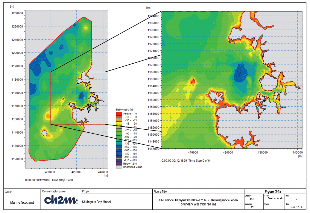
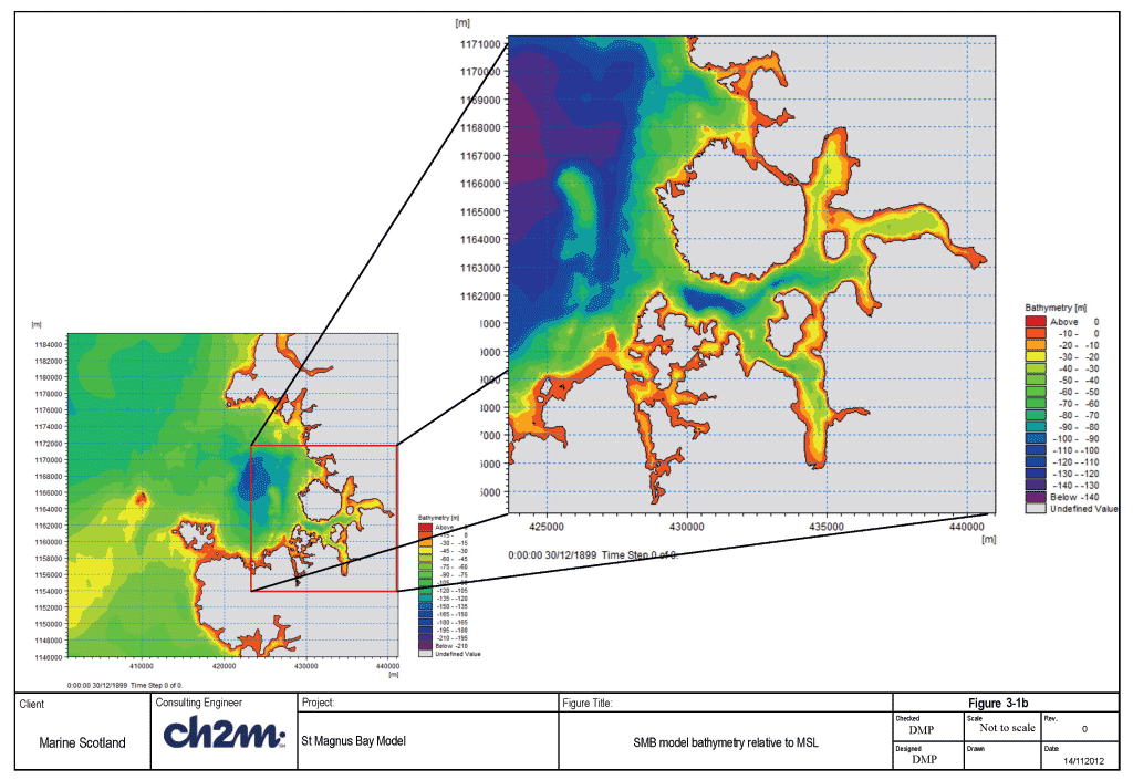
Figure 3-1a shows the extent of the model domain in the left hand frame. The open boundary is highlighted in red. The contours on this and subsequent images are of the model bathymetry which is relative to MSL. Figure 3-1b shows a closer view of SMB in the left hand frame, and a closer view of the eastern part of SMB in the right hand frame.

3.2.2 Model mesh

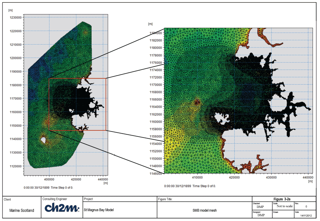
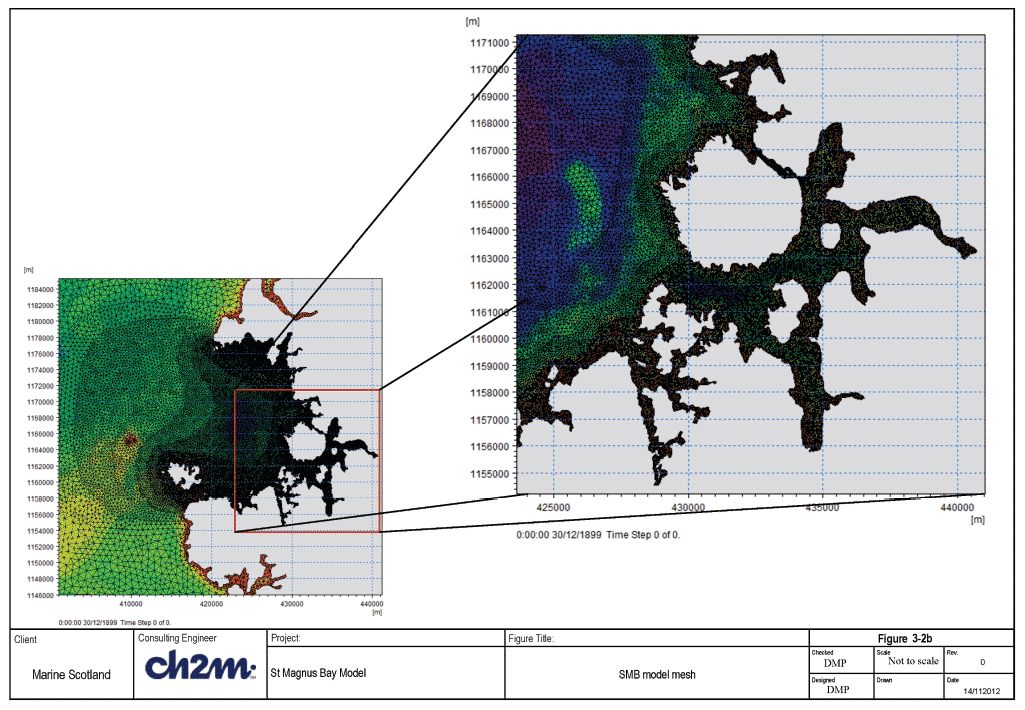
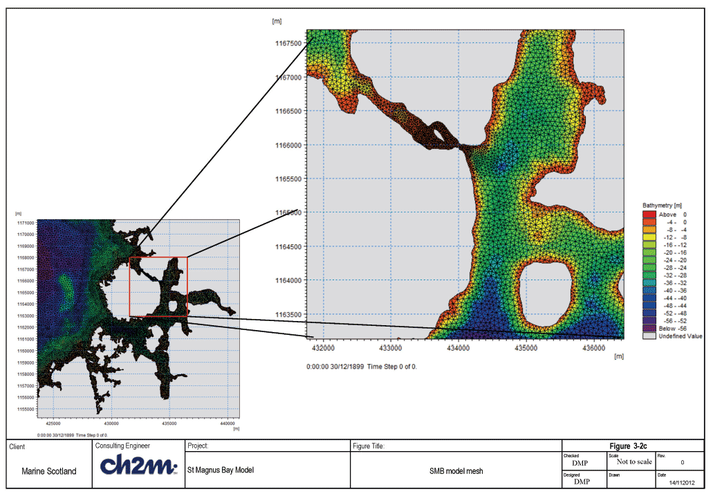
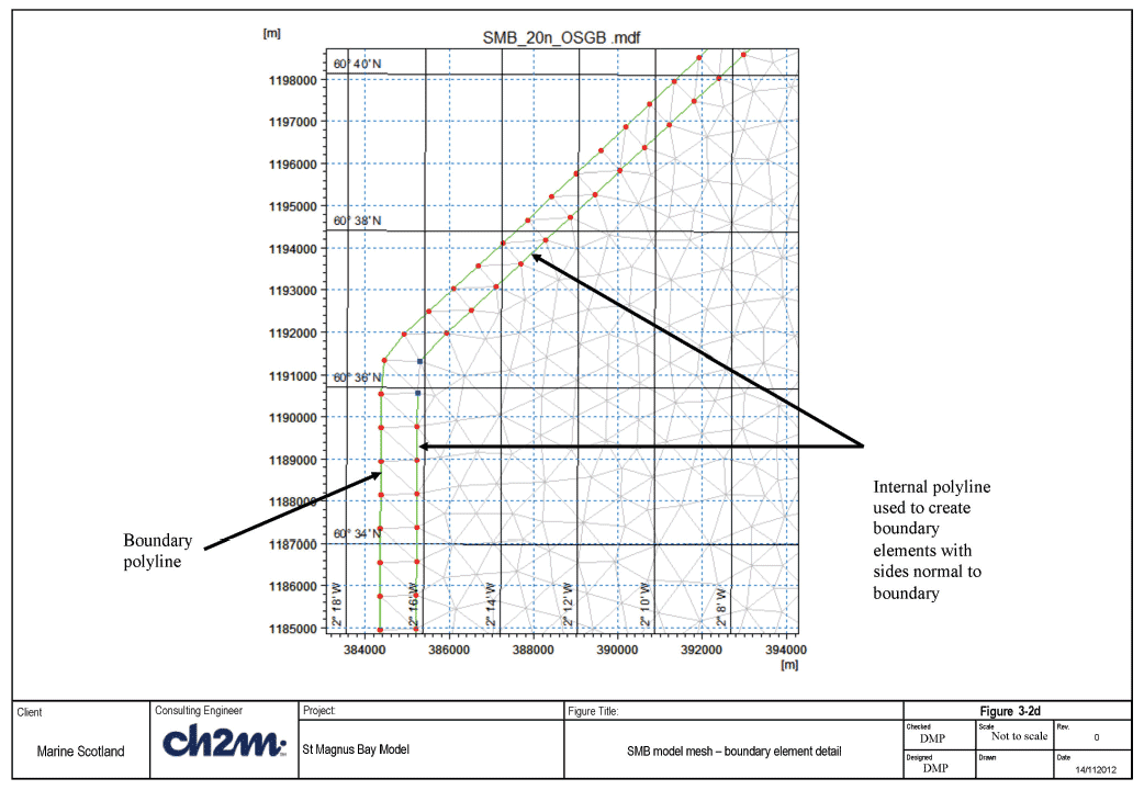
The model mesh was created to provide sufficient resolution within SMB and especially the narrower channels. The mesh was edited to make sure there were no nodes connected to nine or more others. Figures 3-2a-c show the mesh at different zoom levels. Resolution in the offshore region of the model is in the order of 1000m, within the central part of SMB it is 200m, with most of the rest of the area within SMB has a resolution in the order of 50-75m. The channel between Muckle Roe and the mainland has a resolution of 25m in order to be able to resolve the flow through this narrow channel.

It can be seen in Figure 3-2d that there is a polyline inside the outer open boundary. The nodes along this line were defined so that edges of boundary elements were normal to the open boundary. The purpose of this is to reduce interpolation along the boundary for when the model applies water level, currents, temperature and salinity nudging. The simulations undertaken with this model mesh used 10 vertical sigma layers (11 levels), each with an equal 10% proportion of the total water depth.

3.2.3 Boundary data

The nested boundary approach was used to specify the boundary data applied to the SMB model. Water levels relative to MSL, current speeds, temperature and salinity are applied at the centres of all the elements attached to the open boundary (for currents) and all of the attached nodes (water levels, temperature and salinity). These were obtained from simulations of the PFOW model for three specific periods.

Sometimes there can be problems with obtaining boundary conditions from a coarser model and supplying it to a higher resolution local model. The flows within the higher resolution model may be different to the larger scale model due to factors such as mesh size dependent wave celerity, different representations of bed features and physical features such as eddies as examples. FVCOM lets weight factors be applied to the nested boundary nodes and elements, this allows a proportion of the nested boundary values to be factored into the existing values calculated within the model thus reducing and dispersing any sharp gradients and differences. Please see Section 6.4 in the FVCOM manual (Chen et al, 2013) for more detail.

A Matlab script was developed which reads the PFOW results, and creates the SMB nested boundary file. A type 3 nested boundary (which uses the weighting factors mentioned above) was applied to all of the simulations presented in this report using extracted results from PFOW simulations.

The SMB model is run initially with constant temperature and salinity for a short warm-up period, this outputs a hotstart file which contains information about water levels, current speed and temperature/salinity. To reduce the warm-up period for the temperature and salinity, a Matlab script has been used which writes AMM temperature and salinity results to the hotstart file (over-writing the constant values in the hotstart file). This allows the follow-on SMB model hot start conditions to match those applied at the boundary and to have suitable temperature/salinity within the model domain.

3.2.4 Meteorological forcing data

Wind data from the Met Office 12km Unified model was available for certain periods of time but not for the period in 2012 when the MS survey data was recorded. Initially wind for this period was obtained from the MRV Scotia but was subsequently found to be problematic, so wind data from the Met Office UK Waters wave model was used. Data was purchased at 4 points around the PFOW model area and interpolated over the model domain. For further details see the PFOW report (Price et al. 2015). There is no data however for short and long-wave radiation for the period of October 2012 when the calibration data is available. Therefore for this period the model was run for just hydrodynamics alone in order to compare against water level and current speeds. It was subsequently run with time-varying temperature and salinity boundaries but with no further heat input/loss apart from wind as a surface forcing factor; HEATING_CALCULATED was turned off.

The simulation itself (currents/ CTD measurements) was of a short duration (4 days) as the data also covered a short period. Therefore the temperature and salinity comparisons provided in section 3.3.2 are the result of advection/mixing from the initial conditions and boundary inputs of temperature and salinity alone, without any heat exchange with the atmosphere. Without the necessary data this was deemed the best approach. A full baroclinic simulation over the month of May 2009 has been undertaken and compared with a number of vertical profiles of temperature and salinity.

3.2.5 3.4.6 River input

Although rivers are not used in the calibration run they are included in the 2009 validation run. River data was obtained from CEH (received June 2013 and subsequently updated in August 2014 with data in Shetland waters) and encompassed all of 2009 at 15 minute intervals (Shetland had daily average data). This data was processed using a MATLAB tool which determined which mesh node to apply the river flow to. It also moved the location of a river node to the nearest land node if it was connected to two other land nodes in the same element (if connected in this way, then the river flow cannot escape the element and water levels build up artificially too high).

A river namelist file was produced along with a netcdf file for each of the rivers named in it. In simulations with the Shelf model, NOC-L found that reading in over 500 river files impacted upon model performance (input/output overhead). The SMB model was also exhibiting performance issues and therefore all of the rivers were combined into one netcdf file. This, in conjunction with using the latest version 3.1.6 of FVCOM, helped to stabilise runtimes.

The salinity in the river flow was set to 0 psu, and the temperature set to 7 degrees Celsius as this was appropriate for the nearshore temperatures from the AMM model. The river flow is distributed equally amongst all of the vertical layers.

3.3 Flow model calibration

3.3.1 Introduction

Calibration was carried out for October 2012. The data available in October 2012 was collected by MS using the MRV Scotia. This is the best available data for SMB that covers the area offshore and the mouth of SMB. The offshore ADCP location covered one tidal cycle, as did the transects and the CTD measurements which were all recorded within a couple of days of each other. In addition, data recorded at fish farms throughout the Scottish Waters was provided by Alan Hills ( SEPA). This provided 5 locations within the inner part of SMB which proved to be essential, especially as they are located at fish farm sites.

The hydrodynamic model was initially run with 3 vertical layers whilst getting the model to run and to carry out initial sensitivity tests, and then further refined with 5 vertical layers. Subsequently the model was run with 10 layers which is the current form presented in this report.

It was found that the external timestep needed to be 0.25 seconds and Isplit was set as 3.0. Various simulations were undertaken changing the timestep, but due to the constrictions with higher flow speeds and smaller elements in the channel to the north of Muckle Roe it was found it had to be reduced to these values. Horizontal mixing was prescribed with a spatially constant Smagorinsky coefficient of 0.2. Vertical mixing used a constant coefficient of 1E-5, with a Prandtl number of 1.0. Bed roughness lengthscale was set at 0.04m, the same as for the PFOW model. Sensitivity tests were undertaken with varying the bed roughness but current speeds were found to be relatively insensitive to the bed roughness in the deeper water where the MS survey data had been collected, this is likely due to the deep depths and low current speeds.

3.3.2 Offshore water level and current calibration

The data collected by MS included an offshore ADCP deployment for a period of one tide located outside of SMB and a vessel mounted ADCP ( VMADCP) transecting across the mouth of SMB and various vertical profiles using a CTD in and around SMB. Initial comparisons were made against the offshore ADCP measurements which are presented in this section.

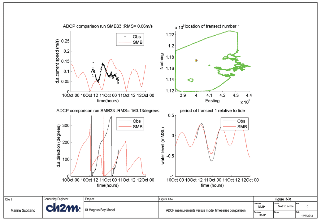
Figure 3-3a presents the comparisons of current speed, current direction, water levels and the location of the measurements within the SMB area. The results presented are from the SMB model simulation SMB_33. A number of simulations preceded this one (simulation SMB_33) which entailed sensitivity tests to bed roughness, horizontal mixing, sponge nodes and boundary configurations. However these results are the ones with the preferred model configuration.

The bed roughness length scale used was a spatially constant 0.04m. No sponge nodes were used as a nesting boundary approach was being used which proved to be stable at the boundaries; earlier versions with water level boundary only did have stability issues which were partially controlled with the sponge nodes.

The top left frame of Figure 3-3a shows comparisons between the observed current speeds (that have been depth-averaged) and the model current speeds at the same location. The location can be seen in the top right frame.

For this simulation, the wind was derived from an interpolation of the wind available from the Met Office wave model, however a sensitivity test (by turning off the wind) showed the model not to be very sensitive to the applied wind at this location and for the period of the simulation. This may in part be due to the comparison being made with depth-averaged currents in deep water. The roughness was the same as that used for the PFOW model.

It can be seen that current speeds are very low for the observed data (black), varying between 0.05 and 0.15m/s. The model (red) produces speeds of a similar magnitude. There also appears to be a phase shift of a couple of hours when examining the peak in the current speeds. This phase shift is also evident in the comparison of current directions. Although the model rotates in a similar manner and in the same direction, the phase shift is apparent. However examining the water levels in the bottom right hand frame the phase shift is not as apparent.

The water level comparisons are reasonable although the tidal range is smaller by 0.25m. No other water level data is available within SMB.

The location of the ADCP is in an area where the flow diverges around Shetland when flowing eastward and converges when flowing westward. Due to the low flow conditions and the location and nature of the divergence/convergence it has proven difficult to get the comparisons closer than those presented. This model takes its boundary conditions from the PFOW model which in turn shows very similar results to the SMB model at this location.

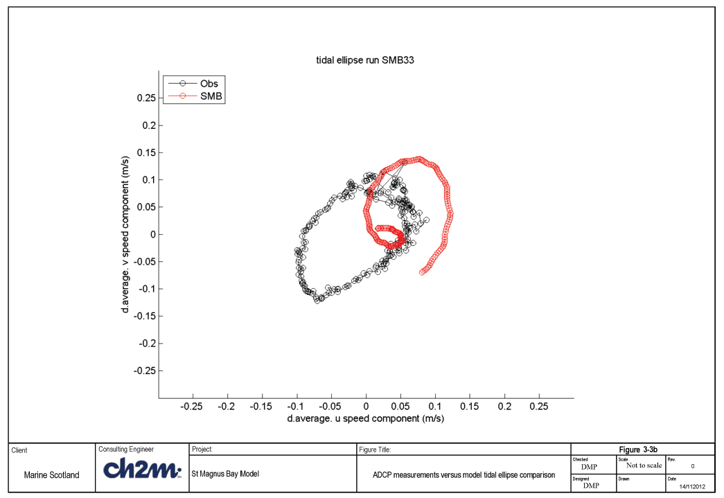
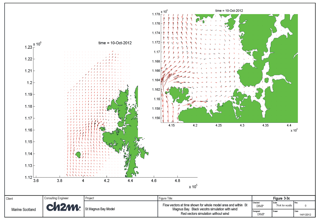
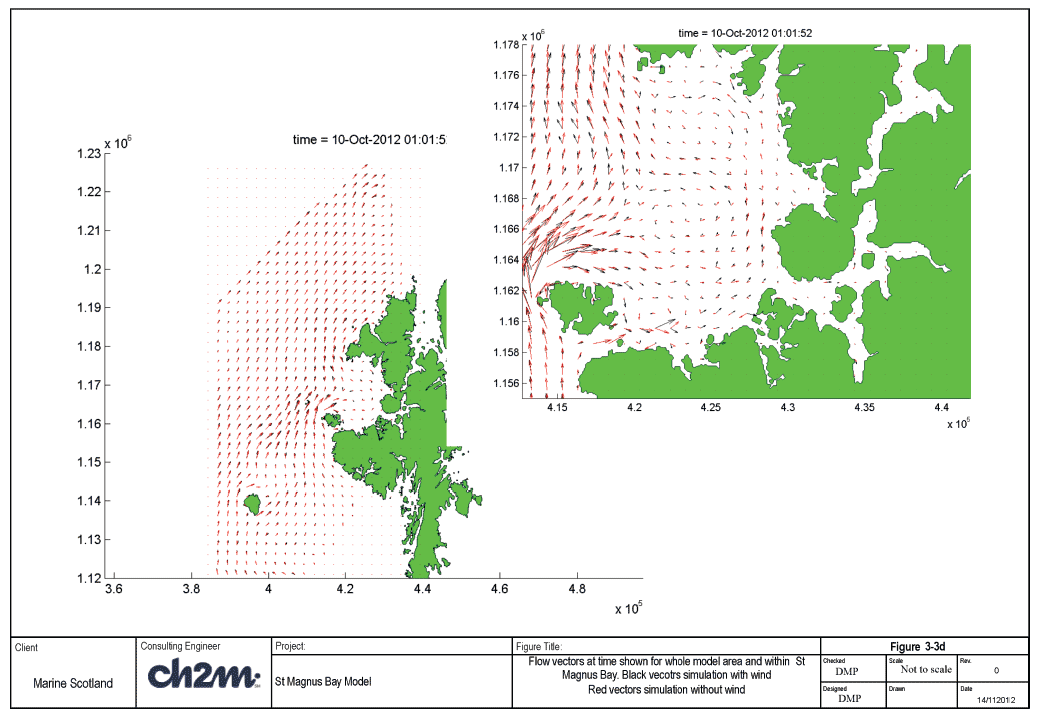
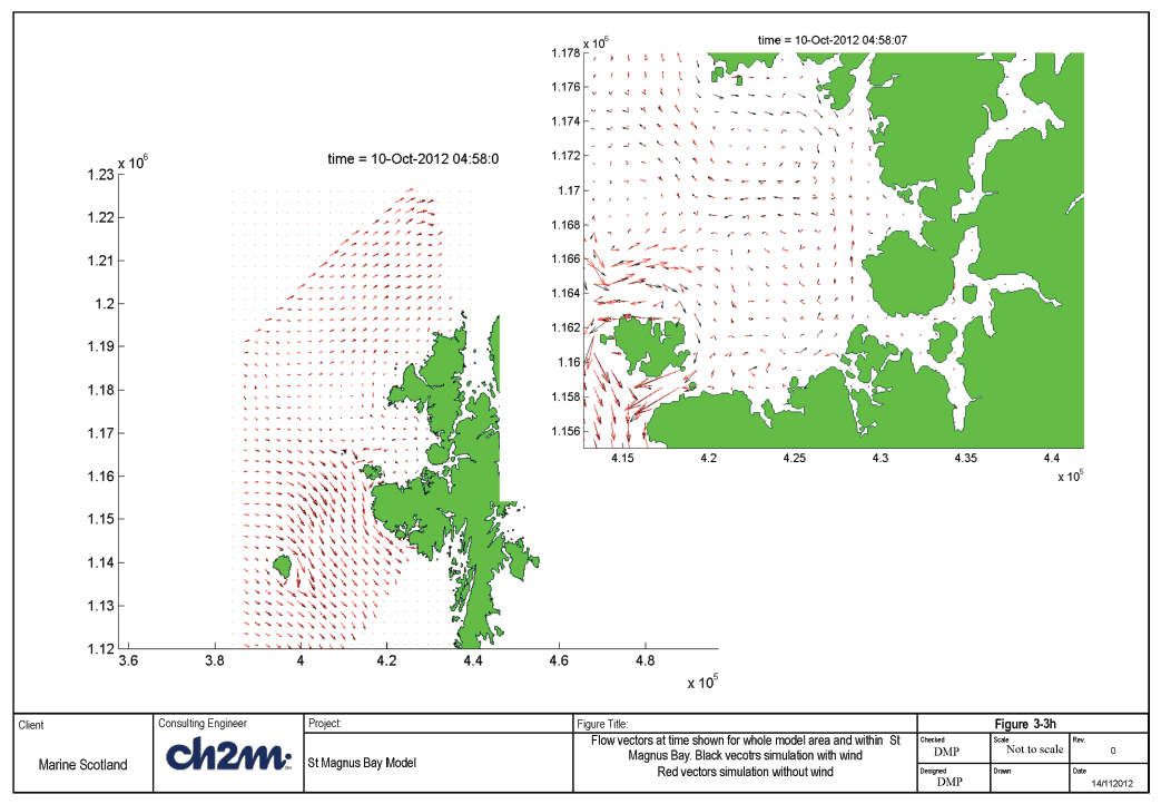
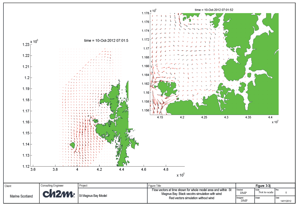
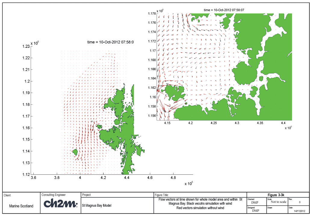
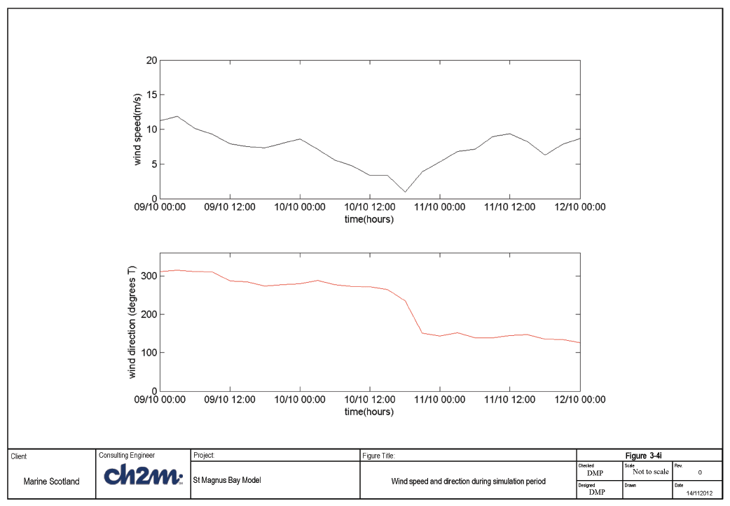
Another way of visualizing the flow conditions and providing a comparison between the model and observed data is to plot the tidal ellipse. This is presented in Figure 3-3b. The general direction of the major and minor axes are comparable however the issue with the phase shift means a better match is not possible for the same period of time. Figures 3-3 c-o show hourly depth-averaged current vectors for the whole model area (left panel) and a close-up of the St Magnus Bay ( SMB) area (right panel). Additionally two sets of coloured vectors are included, the black vectors represent the simulation including the wind (shown in Figure 3-4i) and the red vectors the case without wind. These are provided to help show the nature of the circulation both outside and inside the Bay and how the wind in this case can affect the flow patterns. Outside of the Bay the direction of the current rotates clockwise with the peak ebb and flood flows being orientated west to east. The flow at times is directed across the mouth of SMB, which in turn appears to set up an anticlockwise circulation in the southern part of the bay and a clockwise circulation in the northern part. Whilst this appears to be the case with/without wind it can be seen that flows within the bay are sensitive to wind conditions and therefore wind is an important mechanism in the movement of the water within SMB.

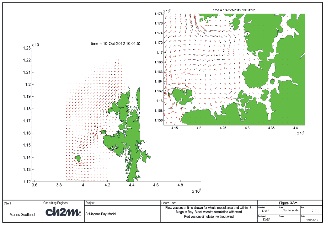
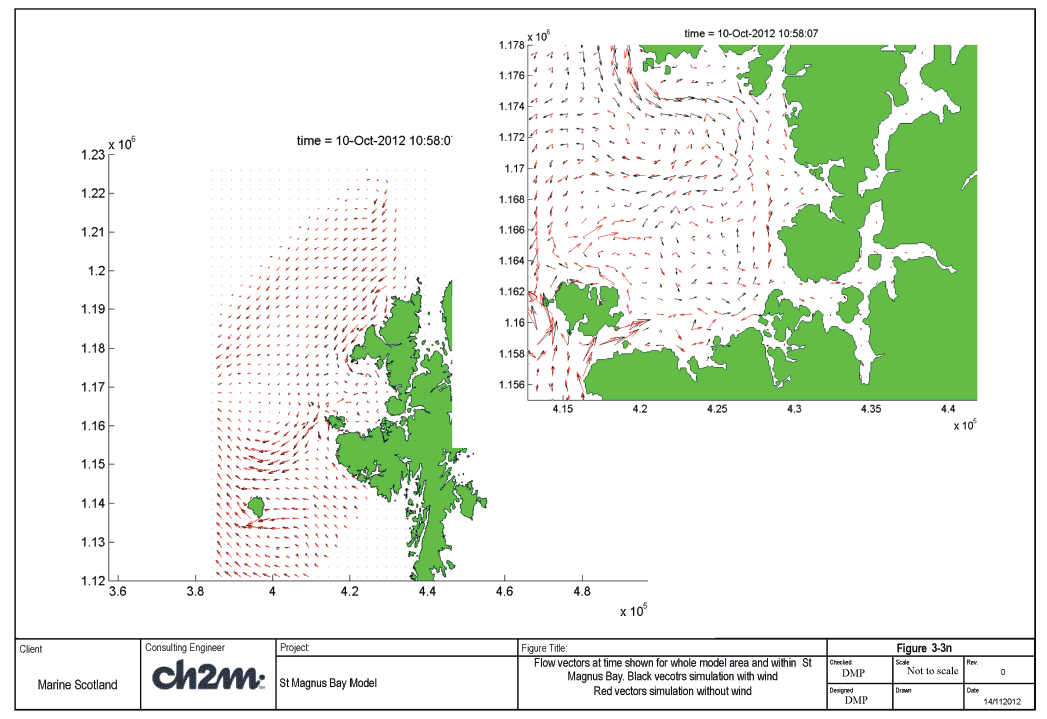
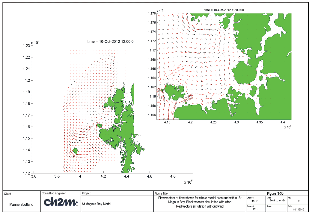
3.3.1 Comparison against VMADCP transects

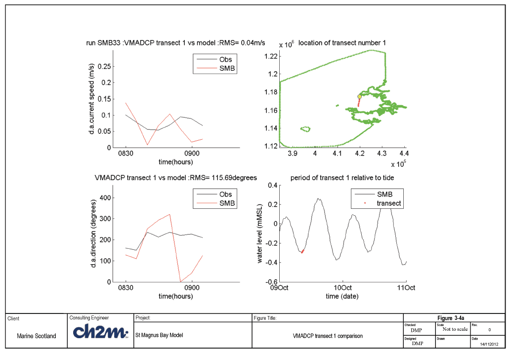
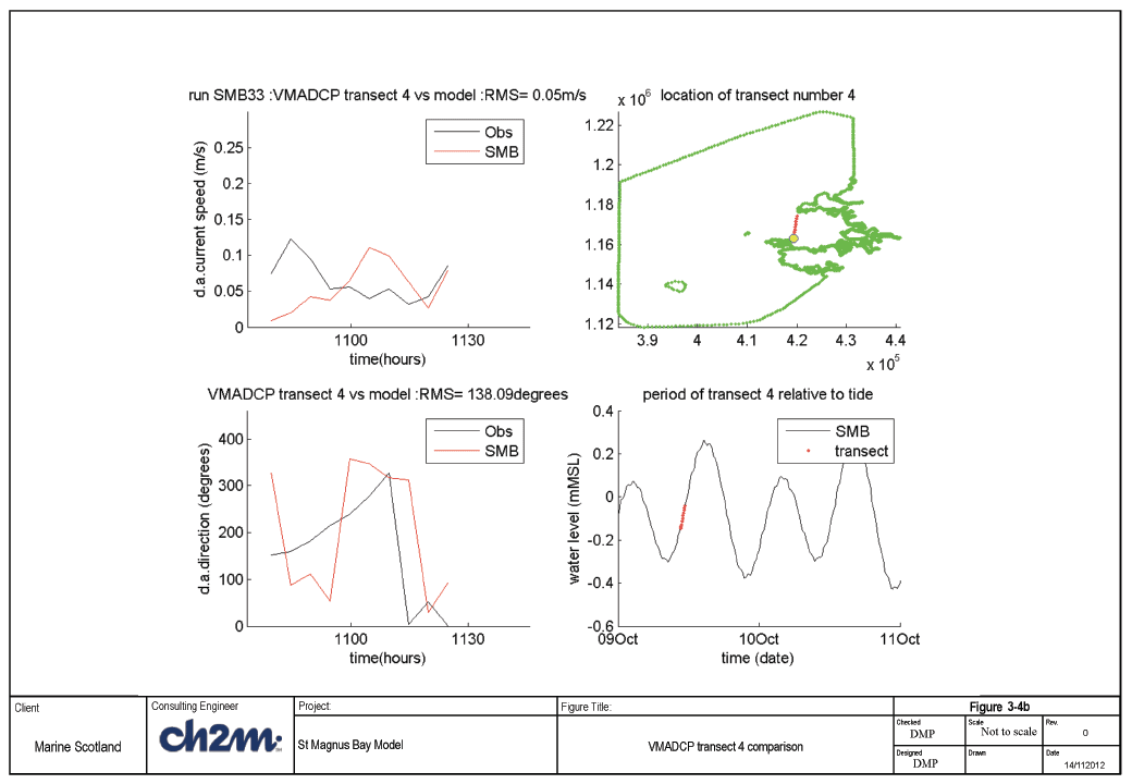
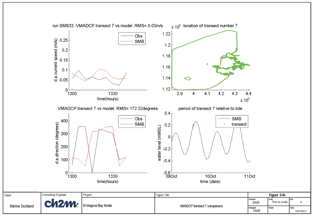
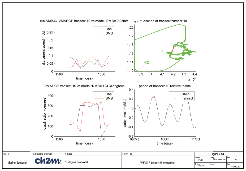
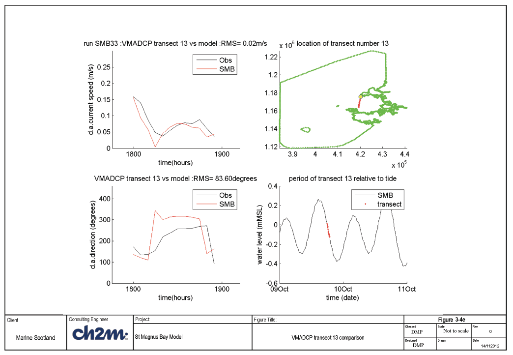
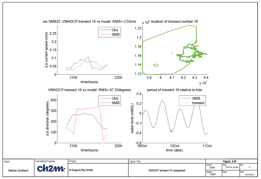
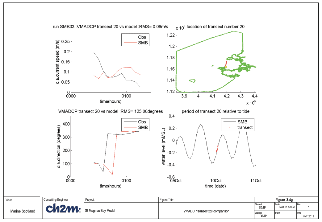
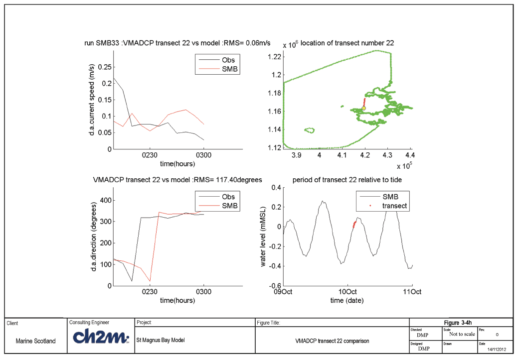
In addition to the offshore ADCP, the MRV Scotia also undertook vessel mounted ADCP ( VMADCP) transects across the mouth of SMB for a complete tidal cycle, this was part of the same survey as the fixed station ADCP measurements used above. A Matlab script was written which reads in the records for each transect, depth-averages them, and then finds the model results for the corresponding location and time. A selection of these transects are presented in Figure 3-4a-h, whilst the remaining ones can be found in Appendix A.

These have been plotted as comparisons of depth-averaged current speed versus time (top left), depth-averaged direction versus time (bottom left), the location and starting point of each transect (top right), as well as the period in the tidal cycle that the measurements were made (bottom right). The simulation ( SMB_33) used to compare against the measurements was the same one used for comparisons against the offshore ADCP data, it therefore includes the effect of wind. The observed transects are indicated by "Obs" in the legend, and the model results by " SMB".

Figure 3-4a shows the current and direction transect compared against the measurements at a time of low water (shown in the bottom right hand frame). Observed current speeds are generally low throughout the transect measurements, rarely going above 0.1m/s (depth-averaged).

The comparisons between model and observed speeds show the model to produce speeds with similar magnitude, and in some cases similar features within the profile. However the phase difference observed offshore at the ADCP location means that a better comparison is unlikely, especially with current speeds that are less than 0.1m/s.

The RMS error is also shown in the title for each frame. It can be seen in Figures 3-4a-h that the RMS error for depth-averaged current speed is in the order of 0.02- 0.06m/s.

Figure 3-4i presents the wind speed and direction (at the offshore ADCP location) applied to the model during the simulation.

3.3.2 Comparison against Fish Farm data

SEPA collated and made available current speed data obtained as part of licensing for fish farms. This data consisted of a minimum of 15 days of recorded current speed at a range of locations in Scotland, including within SMB. Five of these locations were selected because they were distributed throughout the inner parts of SMB.

Table 3‑1 Dates from which the selected fish farm data was collected

Fish farm name	Start time of 15 day observations
BURK	12:00 28 th April 2001
WPL	12:00 28 th February 2001
OLNA	15:30 9 th April 2007
BUD	15:00 20 th February 2002
MUCE	17:00 12 th April 2001

These measurements were made during a range of periods of time and not within the period (or year) of the model simulation. At each location, measurements were made at near-surface, mid and near-bed depths; the model results at the top (layer 1), middle (layer 5) and bottom (layer 10) were used for comparison. Additionally flow speeds were low which meant that the effect of wind proved to have a significant influence upon the current speeds.

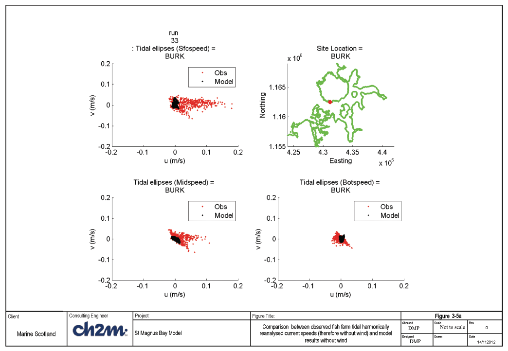
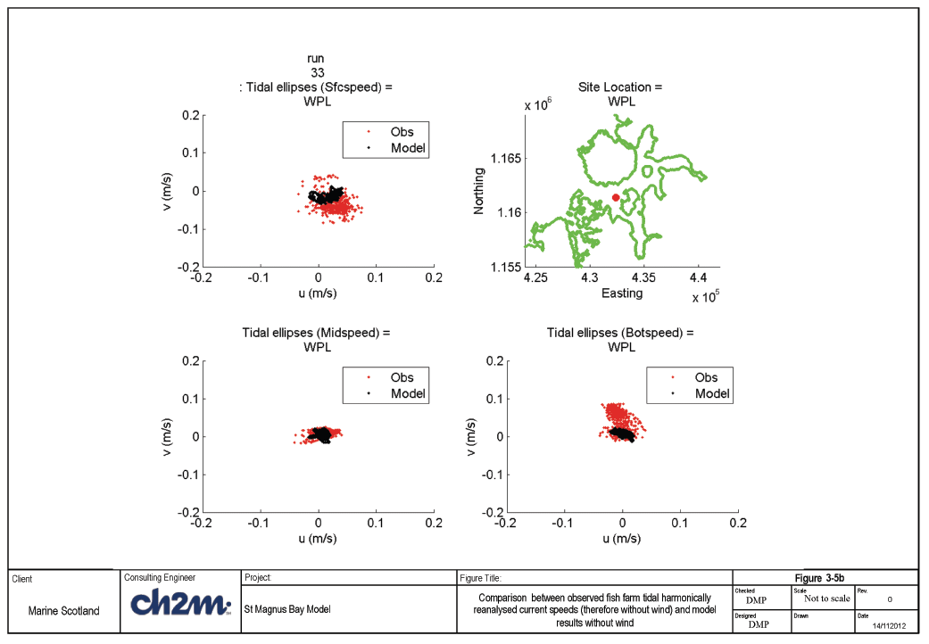
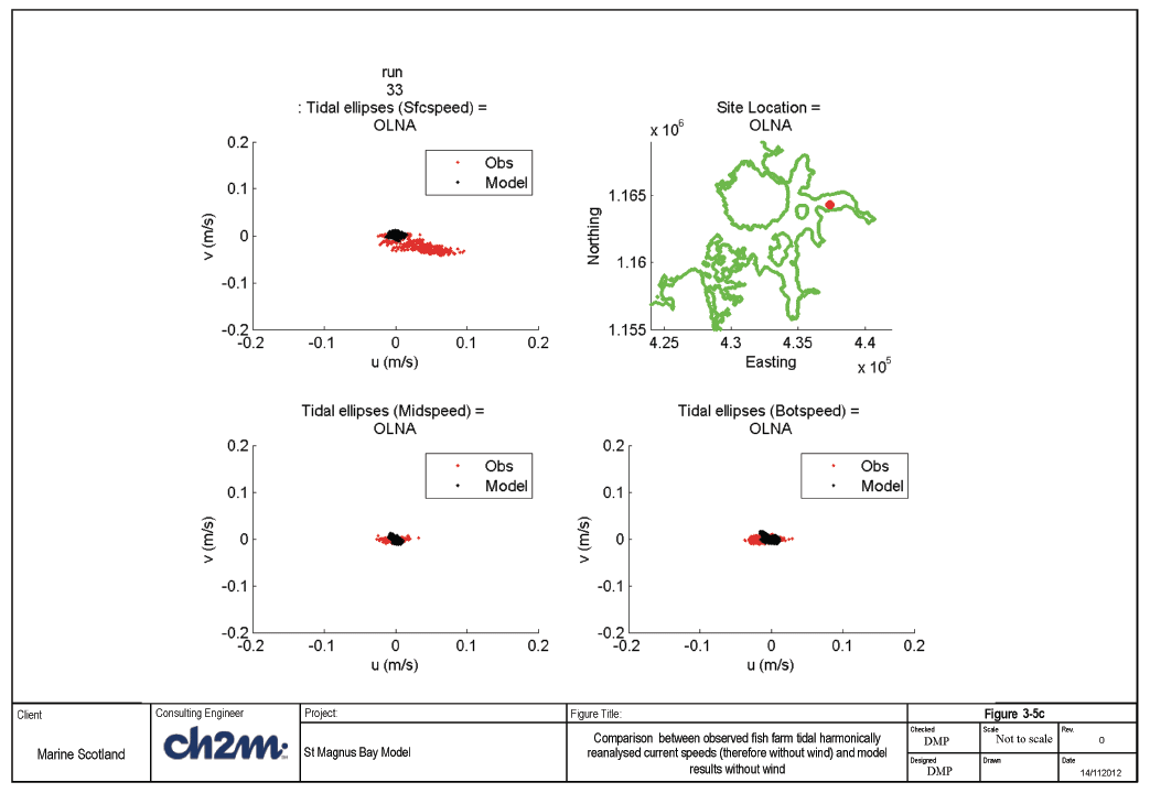
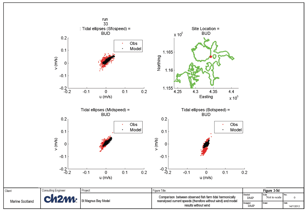
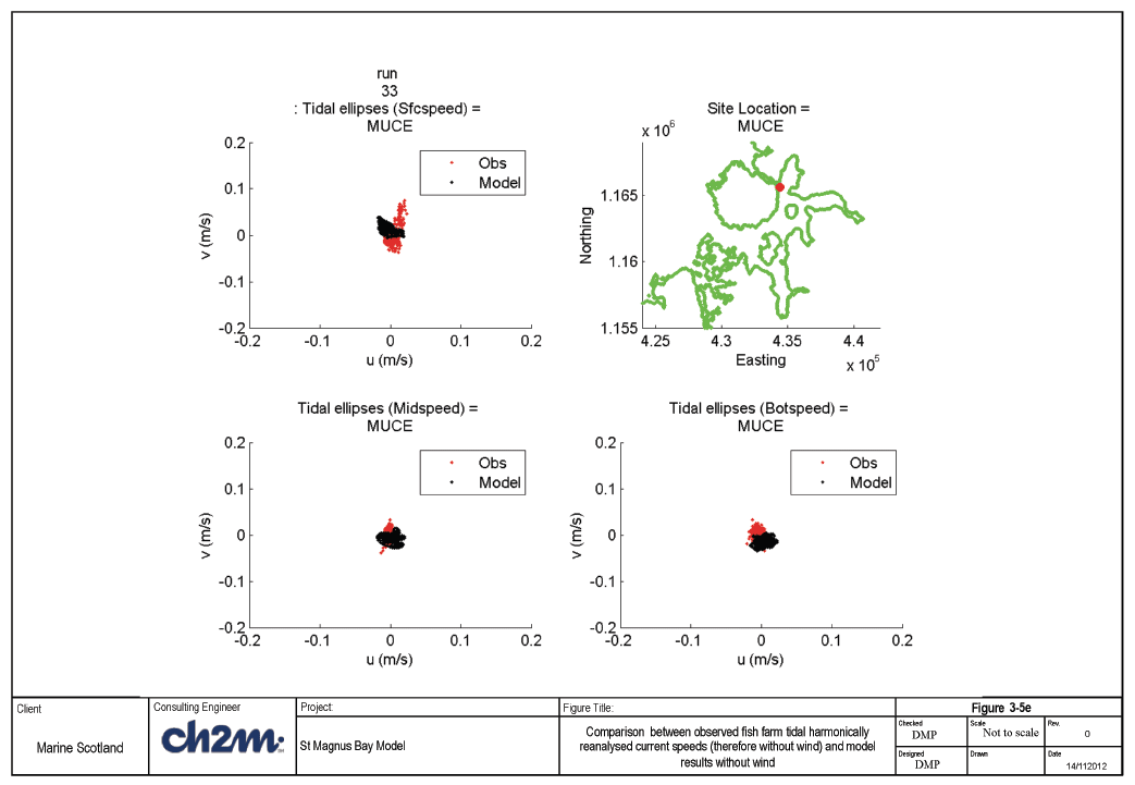
A harmonic analysis of the observed fish farm datasets (15 days) was then undertaken at each of the five locations, and the speed components reconstructed from the constituents at the same times as the model results. Figures 3-5a-e present the near surface (top left), mid (bottom left) and bottom (bottom right) current speed ellipse (velocity components plotted against one another) for the observed speeds in black; the location of the measurement site is shown in the top right frame. The data points plotted in red are the model results from a simulation without wind included.

It can be seen that the model speeds are in general of a similar order to those re-constructed from current observations, with magnitudes of only a few centimetres per second.

3.3.3 Comparisons against observed temperature and salinity vertical profiles - October 2012

As part of the October 2012 survey, MS undertook profile measurements of salinity, temperature and depth using a CTD instrument. These were made throughout the bay and provided a means to compare with the model measurements. Therefore for a simulation of the 10 layer model with wind, was undertaken for the same four day period but with the addition of temperature and salinity boundaries derived from the AMM model. In addition initial conditions of temperature and salinity were also taken from the AMM model. No river flow data or long and shortwave radiation was available for the period of the simulation and therefore the effects of these were not included. This is not an ideal comparison as the simulation is short, however, in the absence of the full met forcing it at least provided a means to test that the general temperature and salinity fields were of the right magnitude and that the data could be used for comparison. A full baroclinic simulation was undertaken for the month of May 2009 (including river inputs) which is reported in Section 3.4.3 below.

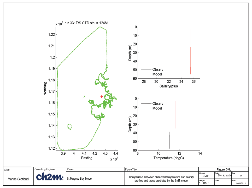
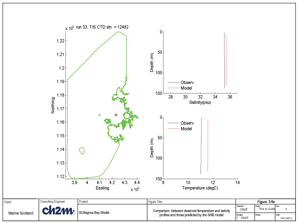
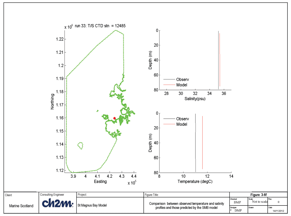
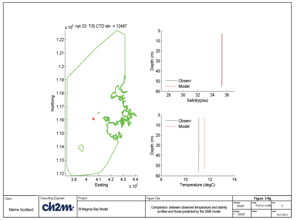
There were 55 vertical profiles within the SMB model domain at which comparisons were made. A small selection of these has been presented to provide a good spatial coverage in SMB; these can be seen in Figures 3-6a-g. In general most of the vertical profiles show the water to be vertically well-mixed, although some evidence of variation with depth can be seen in the observations in Figure 3-6b, with slightly cooler water above 20m depth. Comparisons of salinity between the model and the measured values are close with the model being less than 0.5psu greater than the observed. For temperatures, the model predicts temperatures which are approximately 0.5-0.75 degrees Celsius greater than the observed values. Both are within the tolerance ideally expected from the model. As the model did not include full met forcing, the temperature within the model does not undergo any exchange of heat between the atmosphere and the sea water.

3.4 Flow Model Validation

3.4.1 Introduction

Validation runs were carried out for May 2009 and October 2001. Data was available for May 2009 to validate against temperature and salinity profiles, and October 2001 for validation of current speed against fish farm measurement.

3.4.2 Direct comparisons with Fish farm data at site COLE1

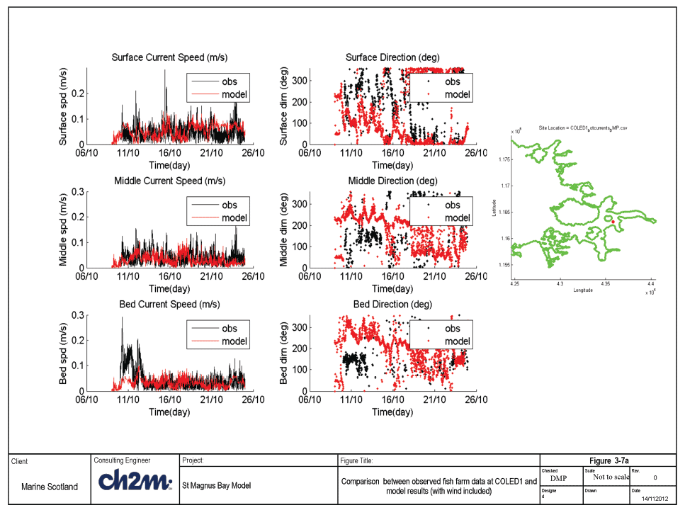
The fish farm data were each collected at different times and locations. However there was a site which coincided with a simulation that had been run for the PFOW model namely October 2001. During this period local wind speed/direction information had also been recorded alongside the currents and was applied throughout the whole model domain as a timeseries. This is an oversimplification but in the absence of other more detailed data was felt to be appropriate.

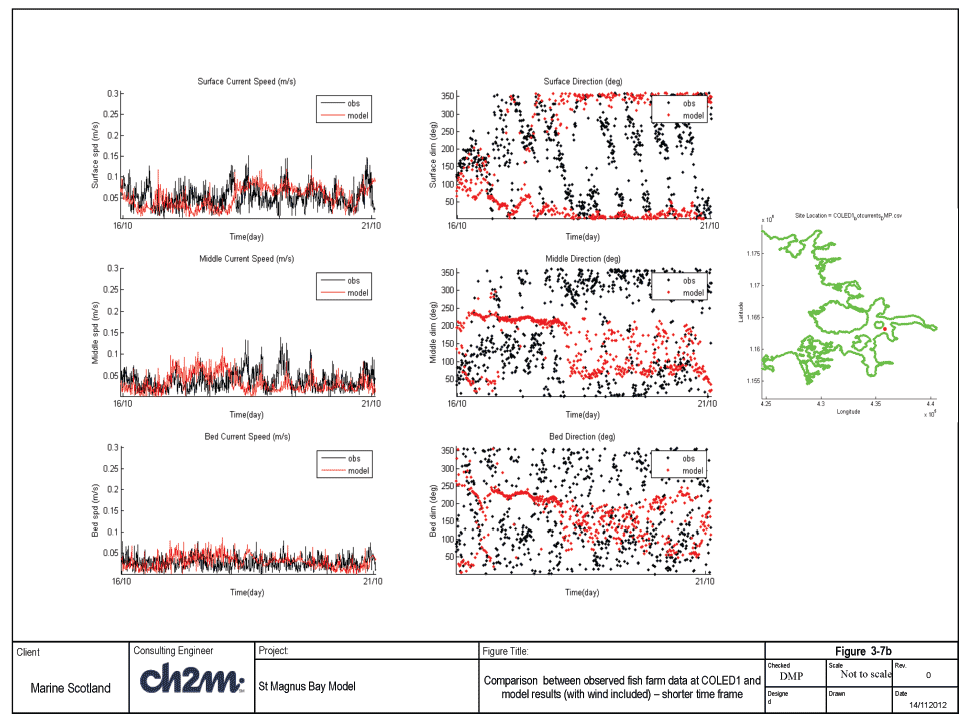
Figures 3-7a and b present the comparisons between the model results and the data, with Figure 3-7b being the same comparison as Figure 3-7a but zoomed in on a shorter timeframe. The top two frames show the surface current speed and direction, the middle two the mid-depth and the bottom two the near bed current speed and direction. Observed current speeds are generally in the region of 0.1m/s although there are isolated periods when speeds at the surface attain speeds of 0.2m/s. Given the low current flows it is very difficult to get an exact match. Examining Figure 3-7b it can be seen that many of the peaks in current speed have been reproduced by the model although not all of them. There are a number of reasons for differences including but not limited to boundary conditions, spatially constant wind from local site (may not be applicable over entire area) and errors in measurements of such low current speeds. Therefore, given some of the possible errors and the low current speed we believe that the model represents the current speeds reasonably well. The current direction comparisons do not appear to be as good although the eye is attracted to all measurements whether current speed is very low or not and so some of the directions may be misleading. The effect of wind appear to be stronger in the model than the observations (surface current sets in a constant direction for several days in the model, while the current appear to rotate in the observations).

3.4.3 Comparisons against observed temperature and salinity vertical profiles - May 2009

In order to validate the temperature and salinity predicted by the model, a longer simulation was required coincident with available data. Such data was found in the BODC archive for four locations outside of SMB but within the model domain. The SMB model was therefore run in baroclinic mode for the period of May 2009 as results from the PFOW model were available towards the end of this time period, thus allowing a good length of time for the model to become warmed up.

Boundary conditions, river flows and meteorological forcing (from the Met Office mesoscale model) were created for the SMB mesh and the simulation undertaken. Some smoothing of the initial few hours of the nesting boundary was required so as not to create a shock within the model when the current speeds were introduced as these are not affected by the iramp smoothing parameter in FVCOM.

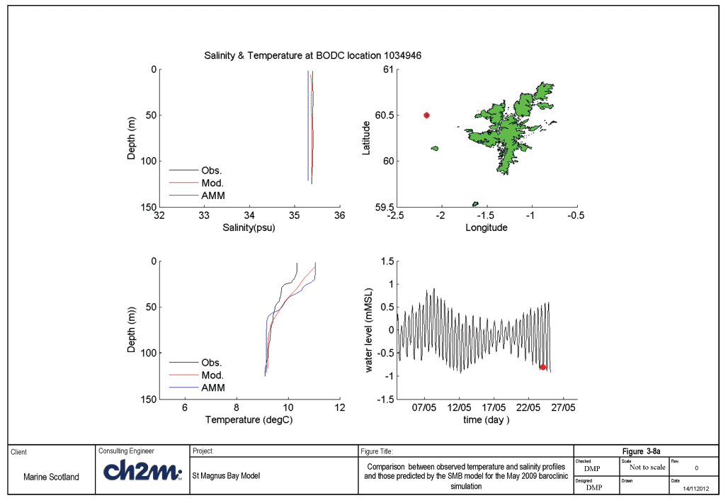
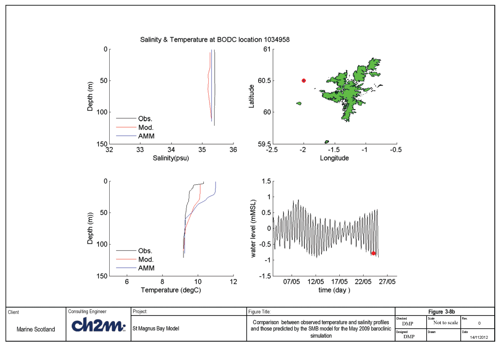
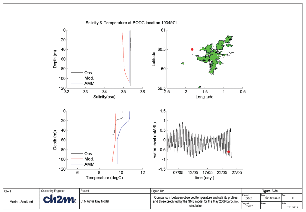
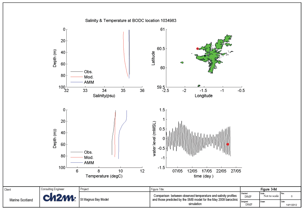
Results from the model in the form of temperature and salinity comparisons with vertical profiles of temperature and salinity are presented in Figures 3-8a-d for locations from west to east towards SMB.

The offshore location (Figure 3-8a) is close to the model boundary and shows a good reproduction of the data and the AMM results. The temperature for the AMM and the SMB model are slightly higher than the observed data in the top half of the water column by almost 1 degree although the SMB model results are closer to those observed. This is also the case for Figure 3-8b, although the salinity can be seen to be very slightly lower than that observed for mid depths although well within the required accuracy. The temperature at the surface and the bed reproduces the observed values closely. Between about 75m and 20m water depth however the SMB model is over-predicting temperatures by just over 0.5 degrees. However the AMM model does this to a greater extent which appears to have translated into the SMB model via the boundary conditions derived from the AMM model.

Figure 3-8c shows that the SMB model is predicting slightly lower salinities than those observed or in the AMM model. This is less than 0.5 degrees however and therefore within the accepted limits. However this may suggest that the freshwater input may be too high. The temperature profile predicted by the model is also shown in this Figure, magnitudes are similar to the observations throughout most of the depth although the higher temperatures in the top 15m of the water column shown in the data is not reproduced. And shows a more mixed water column.

Figure 3-8d shows the same under-prediction of the salinity albeit quite small. The temperature profile however shows the same vertically mixed condition as in the previous Figure, however in this case the data also shows the same feature. This suggests that for this time period the water column is stratified offshore, but closer to SMB it is vertically well-mixed.

3.5 Summary of model calibration and validation

In general, current speeds within SMB are low and are influenced by wind as much as by tides. Comparisons with current measurements outside of SMB have shown the model to have similar magnitude current speeds but turns earlier than observations. Comparison of transects across the mouth of the Bay show the model able to reproduce the magnitude of current speed well, including the structure (especially for direction) along the length of transects; without the effects of wind however, the comparison was not as good suggesting that wind plays an important role. Comparisons of the model flow vector results with and without the wind applied showed differences in the flow patterns within SMB. The current speeds within SMB are therefore sensitive to the applied wind given that tidal current speeds can be low.

Measurements of currents at such low speeds could contain a relatively large error compared with measurements of higher flow speeds. Errors could be of a similar order to the observed current speeds, therefore it would be important to get the predicted current speeds to the same order of magnitude as the low observed current speeds, which has in general been achieved within SMB.

In addition to the tidal ellipse comparisons with the fish farm data, a simulation was undertaken at one of the Fish Farm locations within SMB. This observed data was concurrent with a PFOW model run which provides boundary conditions. In addition to the current measurements, wind measurements were also made at the site. Therefore the simulation also including this local wind which has been seen to be important in the inner SMB region. The results showed that the reproduction of the low speed conditions was achieved along with reproduction of some of the features within the observed speed record. At such low speeds it is likely that accurate wind speed data would prove beneficial and is likely to play an important part in improving upon the comparison with data.

Although limited data was available, the model has shown that it is able to reasonably reproduce the temperature and salinity measured within the model domain including some of the vertical features that are present.

3.6 Flow model simulations

3.6.1 Introduction

This section of the report describes the climatology runs of the flow model for the St Magnus Bay ( SMB) area. The model set up used has been described in the calibration section. The requirement was to produce a six month climatic run, from May to October, based on climatological forcing, representing a typical annual climate. This was carried out using the Scottish Shelf model climatology results as initial conditions as well as for boundary conditions. The input data sets for climatological meteorological forcing and climatological river fluxes used in the shelf model were also used for the SMB model. For a full description of the input data, the sources and how it was processed for climatological runs see the Scottish Shelf Modelling report (Wolf et al. 2015)

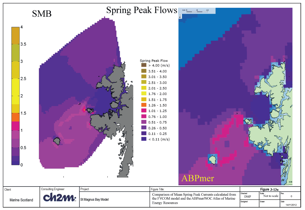
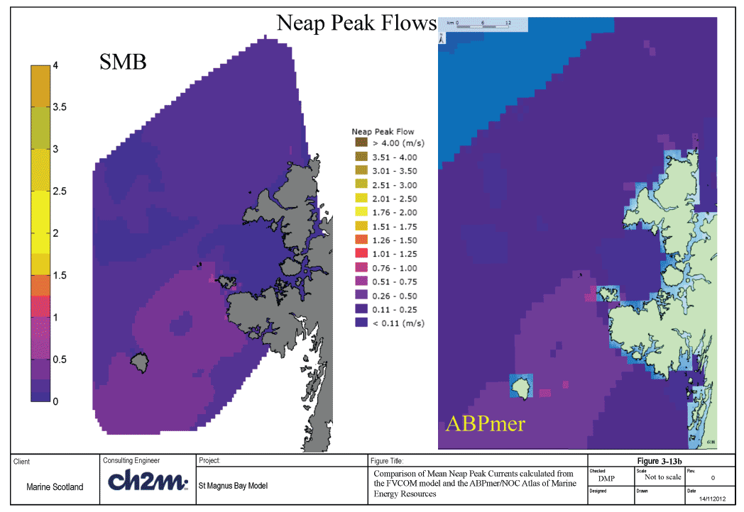
The results from the climatic run were used for particle tracking and to develop connectivity indices. The results have been compared with climatological atlas information for temperature, salinity and currents. The neap and spring tidal ranges and peak flows are also compared with the ABPmer tidal atlas.

3.6.2 Climatology Input Data

3.6.2.1 Boundary conditions

Boundary forcing for water levels (mean yearly tides), currents, temperature and salinity were taken from the Scottish Waters Shelf model climatology results. Hourly results were interpolated on to the nested boundary nodes and elements using a Matlab script. Because the shelf model was run with 20 layers whilst the SMB model has been run with 10 layers it was also necessary to average the current components, temperature and salinity from 20 to 10 layers. This was also carried out in the Matlab script. The decision to use boundary conditions from the shelf model instead of PFOW as in the calibration runs was based on the relative resolution of each model in the vicinity of SMB. The shelf model resolution is higher, therefore the bathymetry in the Shelf model is more consistent with that of the SMB model than that of the PFOW model in this area.

3.6.2.2 River input

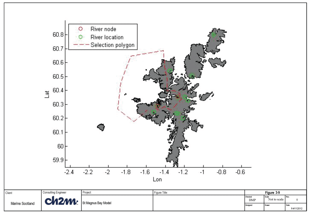
River climatology data was processed by NOC-L from two sources: (i) a reconstructed river climatology derived by reference to the E-HYPE model (126 Scottish rivers, 1980-2012 provided by the Swedish Meteorological and Hydrological Institute, SMHI), distributed across the 508 G2G river discharge locations for the Scottish mainland, as originally provided by CEH for March 2007 - Sep 2010 (see below) (ii) G2G river climatology (1962-2011, 577 rivers) provided by CEH in August 2014 and updated in October 2014. For full details of how the river data was reconstructed to give climatological daily averages, see the Scottish Shelf Modelling Report (Wolf et al. 2015). Only 2 of these rivers fall within the SMB model domain. The rivers were processed in the same way as those for the baroclinic calibration model runs. Figure 3-9 shows the location of the rivers and the location of the nodes the rivers were applied at and the average monthly discharge in cumecs is given in Table 3‑2.

Table 3‑2: Average monthly river discharge into St Magnus Bay in cumecs.

Average monthly river discharge(cumecs)
	River 5	River 8		River 5	River 8
January	0.58	0.58	July	0.09	0.06
February	0.45	0.44	August	0.15	0.11
March	0.38	0.37	September	0.31	0.28
April	0.21	0.17	October	0.46	0.45
May	0.10	0.07	November	0.59	0.60
June	0.08	0.05	December	0.58	0.58

3.6.2.3 Meteorological forcing

Met forcing data for the climatological simulations were interpolated on to the SMB mesh from the Shelf model met forcing input files at 6 hourly intervals. The met forcing was derived by NOC-L from ECMWF ( ERA-40 and ERA-Interim, licence granted). The ERA-interim data cover 1989 - present, and ERA-40 data cover 1957 to 2002. These data were processed to derive monthly mean wind-stress, pressures, heating and "evaporation minus precipitation" for the period 1981-2010, to match the boundary forcing period.

The met forcing were derived as monthly means, which were specified at the middle of the month i.e. mean February data were applied at the middle of February; then mean March data were applied mid-March etc. The data are then linearly interpolated to 6-hourly smoothed forcing data for each grid-point in the FVCOM model. For full details see the Shelf Modelling report (Wolf et al. 2015).

3.6.3 Validation

3.6.3.1 Temperature and Salinity Comparisons

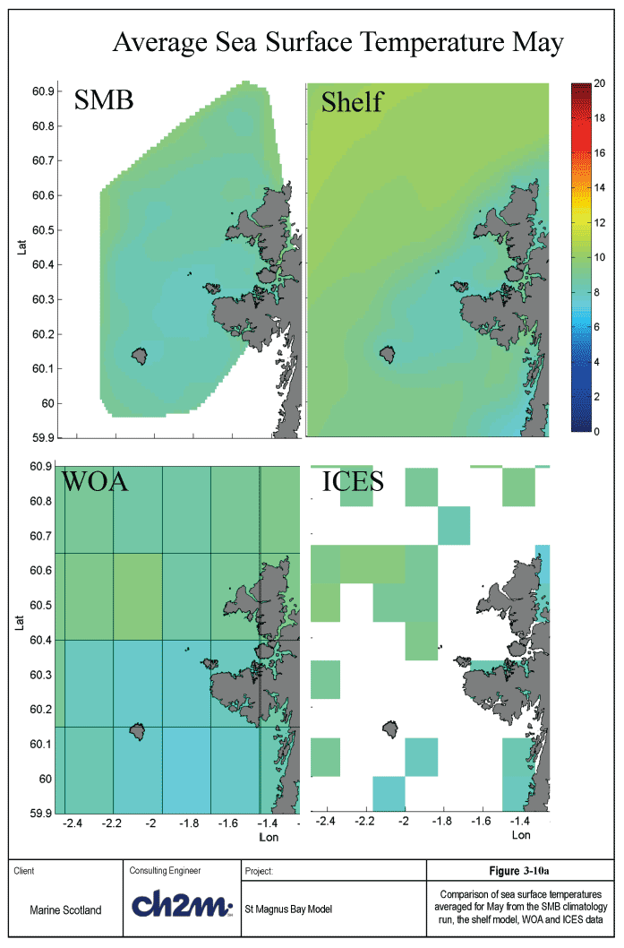
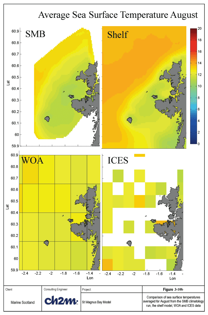
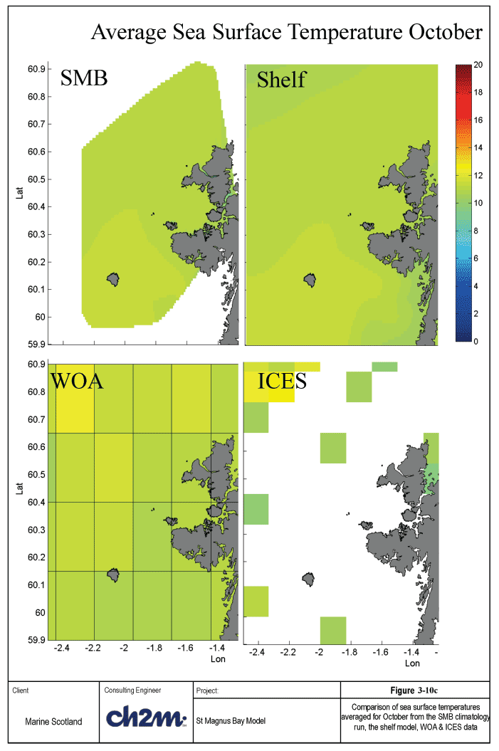
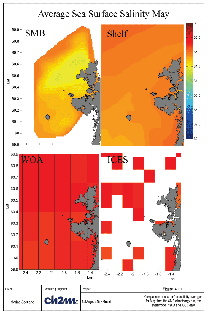
Average monthly sea surface temperature ( SST) and sea surface salinity ( SSS) observations are available from two sources:

1) The ICES (International Council of the Exploration of the Sea) dataset ( http://ocean.ices.dk/HydChem) gridded and averaged for 1960-2004 (45 years) by Jason Holt ( NOC-L). Data are also available from the NOAA/ NDBC World Ocean Atlas (2013);

2) The WOA (World Ocean Atlas) http://www.nodc.noaa.gov/OC5/woa13/) based on over 100 years of observations interpolated on to a 0.25° resolution grid.

These datasets are used for qualitative comparison with the SMB FVCOM results for May, August and October. The resolution of the WOA and ICES data is very low in relation to the model area. Unfortunately no other higher resolution data of SST and SSS are available, therefore the results from the shelf model are also presented.

Figures 3-10a-c shows the comparison of the data sets for SST. Comparison with the WOA and ICES data give good general agreement with the SMB SST. Comparison with the shelf model shows the SMB model gives slightly lower temperature in May and August.

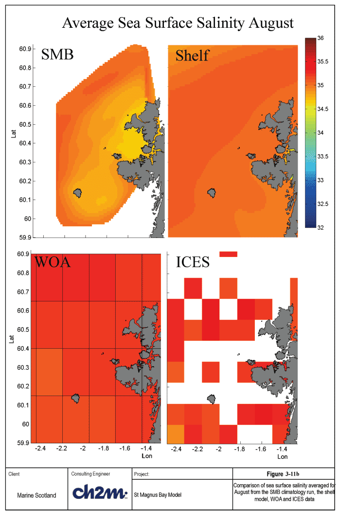
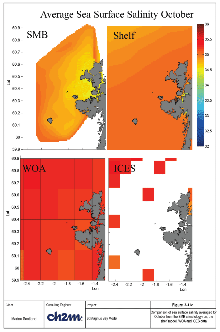
Figure 3-11a-c shows the SSS comparisons. Results from both the shelf model and the SMB give lower sea surface salinities than the WOA and ICES data. The comparison between the Shelf and SMB models show some spatial variations in SSS. Around the boundary of the SMB model result match well however inside the model the salinity is lower than the shelf. This may be due to one of the river inputs not being included in the shelf model. This can be explained by the lower resolution of the Shelf model in the estuary in SMB and the method used to identify the river input locations. As the shelf model does not resolve the estuary the nearest node to the river discharge location in the shelf model was on the east coast of Shetland, not in SMB.

3.6.3.2 Mean Spring/Neap Tidal Range

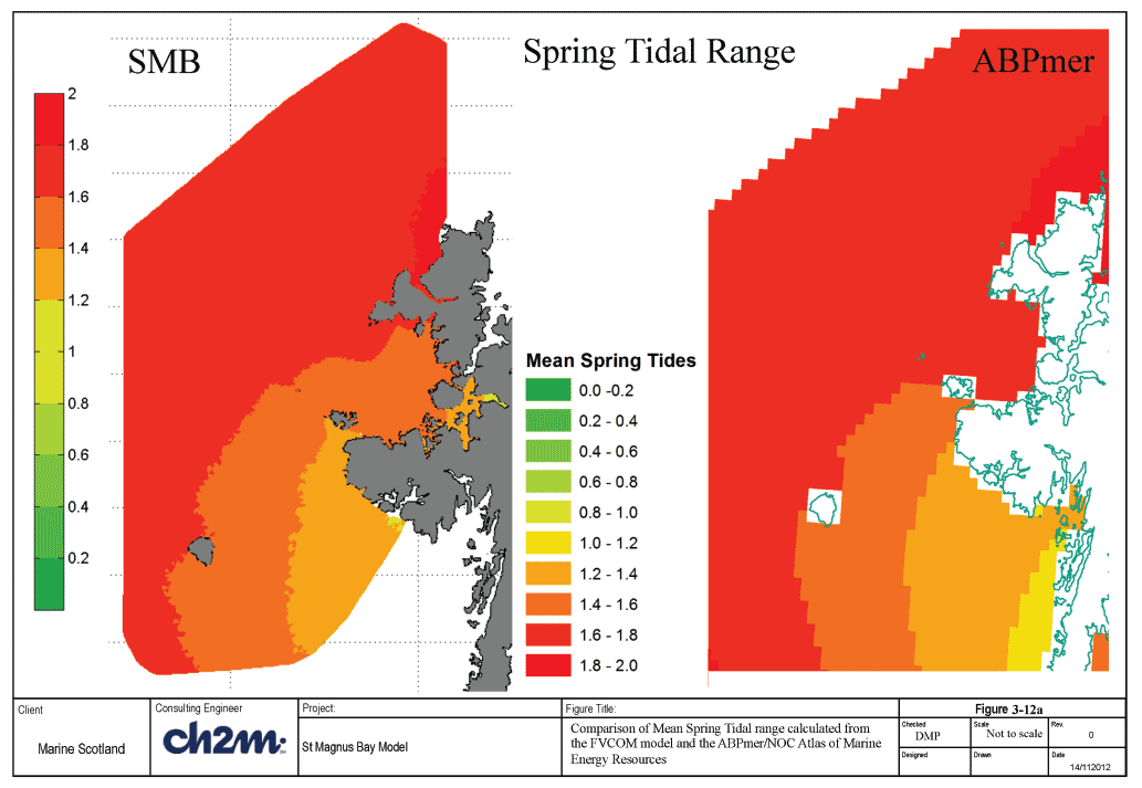
Mean spring tidal ranges have been computed directly from the two principal semi-diurnal components M ₂ and S ₂ based on the following equations from Pugh (1987):

mean high-water springs = Z ₀ + (H _M2 + H _S2)

mean low-water springs = Z ₀ - ( H _M2 + H _S2)

spring tidal range = mean high-water springs - mean low-water springs

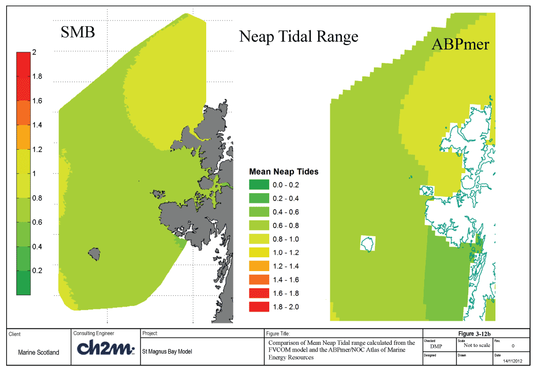
Values for these constituents were obtained from a harmonic analysis of 60 days' worth of data from the SMB climatology run (30/06 - 28/08). These harmonic components control the timing of the spring-neap cycle, and their combination is considered to give a good measure of average spring (and neap) tides. The data was also used to calculate the mean neap tidal range as:

mean high-water neaps = Z ₀ + (H _M2 - H _S2)

mean low-water neaps = Z ₀ - (H _M2 - H _S2)

neap tidal range = mean high-water neaps - mean low-water neaps

A map of the mean spring results are shown, along with the equivalent tidal range from the ABPmer / NOC Atlas of Marine Energy Resources ( http://www.renewables-atlas.info/) in Figure 3-12a. The corresponding plots for mean neap tidal range are shown in Figure 3-12b. The figures show good agreement between the SMB results and the ABPmer Atlas for both spring and neap tidal ranges.

3.6.3.3 Mean Spring/Neap Currents

Mean peak current speeds have been calculated from a harmonic analysis of 60 days (30/06 - 28/08) of depth averaged tidal velocities, from the SMB climatology run. In line with the methodology used for the ABPmer / NOC Atlas, a mid-depth velocity was used for the calculations. The east and west components of velocity were analysed using T_TIDE to give the M ₂ and S ₂ amplitudes and phases. These were in turn analysed to give the semi-major axis amplitudes for each ellipse. The mean peak spring current was then computed as:

mean peak spring current = amplitude semi-major axis M ₂ + amplitude semi-major axis S ₂

The mean neap spring current was computed as:

mean peak neap current = amplitude semi-major axis M ₂ - amplitude semi-major axis S ₂

A map of the results for mean spring current is shown, along with the equivalent peak currents from the ABPmer / NOC Atlas of Marine Energy Resources, in Figure 3-13a. Corresponding plots for the mean neap current are shown in Figure 3-13b. Despite the difference in the resolution between the SMB model and ABPmer tidal atlas the results show good agreement in terms of magnitude and spatial patterns for both the spring and neap peak tidal currents.

3.6.3.4 Residual Currents

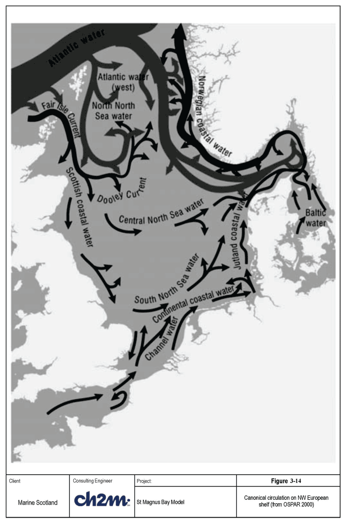
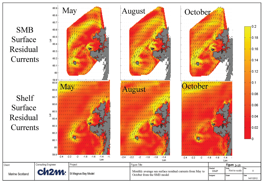
Data regarding the residual currents around St Magnus Bay is not available at a suitable resolution to make comparisons with the SMB model results. Figure 3-14 shows the Canonical circulation on the NW European shelf from OSPAR (2000). It shows that the dominant feature in the vicinity of SMB is the northeast flow of Atlantic water to the west of Shetland. Comparison of the residual current from the shelf model with the SMB model for May, August and September are shown in Figure 3-15. The general pattern spatial and temporal variation in the residual current seen in the shelf model are replicated in the SMB model. Residual flows to the northeast, outside of the bay and clockwise circulation of residuals around Foula. However the residual speeds are consistently higher in the SMB model.

3.6.1 Seasonal Variations

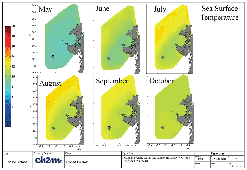
Seasonal variations in sea surface temperature, salinity and residual currents are shown in Figure 3-16 to 3-18. The SST is at its lowest in May approximately 9°C, at this time the SST is also uniform across the model domain. The increase in temperature during the summer moves in from the boundary of the model. Temperature reaches a maximum of around 14°C in August off shore of the Bay. The temperature reduces through September with temperatures becoming uniform again in October.

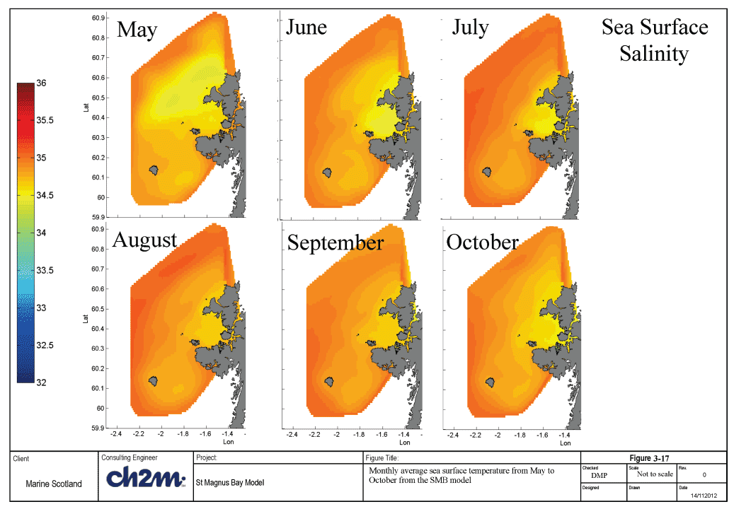
The SSS shows spatial variations from May to October with lower salinity water closer to land during all months. Overall SSS is highest in July and August and lowest in May and October (Figure 3-17). The seasonal variation are not very strong, this may be due to the low input of fresh water from rivers. The fresh water input into St Magnus Bay is low therefore variations in temperature and salinity are likely to be controlled by the temperature and salinity of the Atlantic Waters and the current patterns in the vicinity of the Bay.

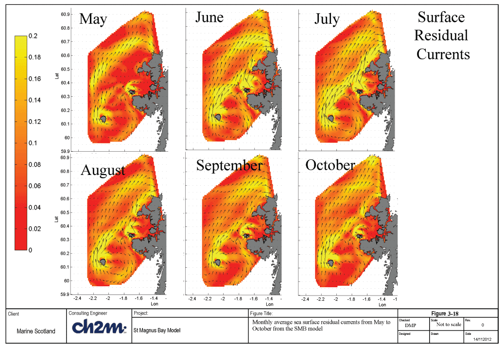
The location of residual current flows show little seasonal variation, the main features being a northeast flow to the north of the Bay and a clockwise circulation around the Island Foula, extending to the west coast of Shetland. However the strength of the currents do vary. Residual currents are at their weakest in May increasing to a maximum in July and reducing again toward October (Figure 3-18).

3.6.2 Summary

Model runs have been carried out to reproduce the hydrodynamic conditions in St Magnus Bay corresponding to the climatology during the period May to October. The input data used was taken from the Shelf Model for boundary conditions, CEH G2G data for rivers and ECMWF averaged data for the meteorological forcing. The model was run for six months, the results have been compared with sea surface temperature and salinity climatological data sets and residual currents for the months of May, August and October. These results compared well with the available data. Only weak seasonal variations in sea surface temperature, salinity and residuals were observed.