Scottish Marine and Freshwater Science Volume 5 Number 5: Identfying a Panel of Single Nucleotide Genetic Markers for River Level Assignments of Salmon in Scotland

Results

Hierarchal splits and SNP ranking

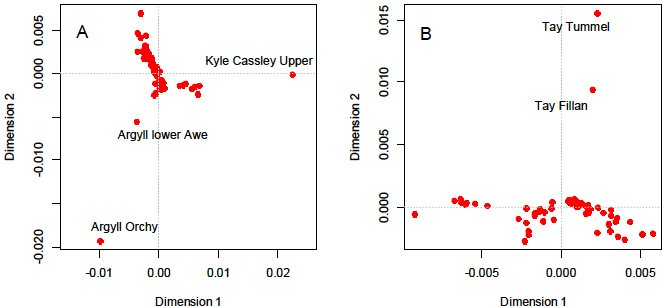
Figure 4 MDS plot of pairwise DA of all sites.

Figure 4A details the pairwise DA relationships between the various sites across the whole of Scotland. Three sites can be seen that fall outwith the central grouping of sites and were removed from the next stage of the analysis. DA was recalculated and the relationships re-plotted in Figure 4B. Two more sites are seen to fall outwith the central grouping and were again removed.

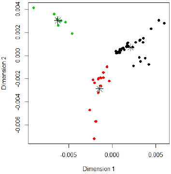
Figure 5 MDS plot of all pairwise DA of all sites after removal of outliers showing how the sites split into 3 groups using K-means clustering. Black are east and south group ( ES), green are Kyle of Sutherland group ( KY), red are north and west group NW).

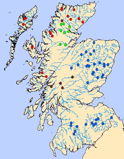
Figure 6 Map showing the top level regional groupings of sites as defined by K-means clustering. Green are Kyle of Sutherland group ( KY), blue are east and south group ( ES), red are north and west group ( NW), brown are the outlier sites.

Figure 5 details the split of sites into the 3 groupings identified using K-means clustering. Fig 5 shows that these 3 clusters represent regional genetically similar site groups that also are related well to geographic location. Due to the particular interest of being able to distinguish fish at the first level which originate from the NW or KY and ES groups the first SNP ranking procedure was carried out using the NW group as one regional assignment unit and the KY and ES groups as the other ( SNP Ranking 1 on Figure 2). SNPs were thus identified which had greatest power in splitting up these two units.

As described in Figure 2 the second level analysis was focused on being able to differentiate between fish which originate from the KY and ES groups and so the second level analysis was performed on these data only ( SNP Ranking 2 on Figure 2).

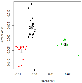
Figure 7 MDS plot of all pairwise DA of KY and ES sites showing how the sites split into 3 groups using K-means clustering. Red are south group (S), green are Kyle of Sutherland group ( KY), black are east group (E).

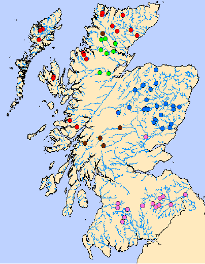
Figure 8 Map showing the regional groupings of sites as defined by K-means clustering. Green are Kyle of Sutherland group ( KY), blue are east group (E), pink are south group (S), red are north and west group ( NW), brown are the outlier sites.

As before, Figure 7 shows that the KY group are separated from the remaining fish, but in this second stage analysis the previous ES group is seen to split into 2 further groups, one associated with the east coast and one with the south of Scotland on both coasts. Again as is shown in Figure 8 the groupings are geographically consistent apart from a single site on the Tay which seems to fall into the S regional group.

After identification of the E and S split, a further round of SNP ranking and identification of those most powerful in separating these two groups was performed ( SNP Ranking 3 on Figure 2). Once this was completed SNP ranking were available which allowed identification of loci which had the most power in separating all regional assignment units identified. The next stage of the process was in areas where there was sufficient river coverage, and which were of particular interest to be able to assign fish to the river level ( i.e. east coast and southern regions) further SNP ranking was performed separately on the data from the different regional assignment units, this time focusing on ranking the SNPs according to their ability to differentiate rivers ( SNP Ranking 4, 5 and 6 on Figure 2).

The outcome of the procedure described above was 6 sets of ranked SNPs each detailing the most powerful loci for separating the particular regions or rivers upon which their ranking was based. The top 48 SNPs from each ranking set were taken and combined into a single screening panel of 288 SNPs. Where SNPs were duplicated in more than one ranking set (33 loci), the next on the list was add as a substitute.

Assignment accuracy to region

At each stage of the hierarchical ranking stages assignment, power was analysed by assigning fish back to the particular split under investigation using the HS data set. From each ranked list, assignments of the HS to the TS data sets were performed with varying numbers of SNPs (12, 24, 48, 96, 192 and 288 SNPs) to determine assignment accuracy. Correct assignments to reporting group (region or river) were determined using all assignments, and also using an illustrative assignment cut-off score of 80 which achieves a balance between assignment vigour ( i.e. only assigning fish with a strong assignment score) and the number of fish assigned ( i.e. not being too strict as to only leave very few fish assigned).

Assignments to the three top level assignment units are shown in Figure 9. As expected, the more SNPs that are used the greater the accuracy of the assignments up to an asymptote beyond which little if any extra power is obtained. The full HS set can be seen to be very well assigned with an accuracy of between 90 to 100% correct with 288 SNPs. If focus is made on just the HS data from complete sites that were removed from the data-set before SNP ranking but which had other sites in their river represented in the baseline then the accuracy is seen to be much the same as the full HS set (which of course includes half the data from all sites). Finally, if the data from rivers not represented in the baseline and which were not included in the SNP ranking procedure is examined, a small drop in accuracy is seen with

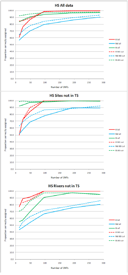
Figure 9 Proportion of fish assigned to a reporting region that are correctly assigned with varying numbers of SNPs to top levels regional assignment units: KY is Kyle, NW is North and West, ES is East and South. Solid lines are all data dashed are assignments using a cut-off value of 80 for the assignment score.

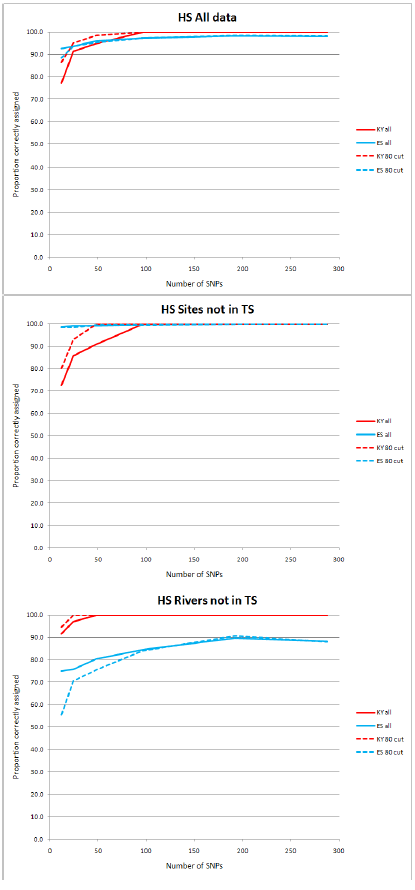
Figure 10 Proportion of fish assigned to a reporting region that are correctly assigned with varying numbers of SNPs to the first East and South coast regional split level: KY is Kyle, ES is East and South. Solid lines are all data dashed are assignments using a cut-off value of 80 for the assignment score.

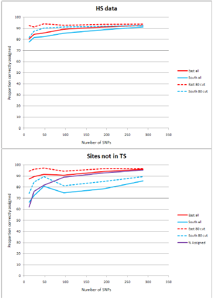
Figure 11 Proportion of fish assigned to a reporting region that are correctly assigned with varying numbers of SNPs to the East and south coast regional split level. Solid lines are all data dashed are assignments using a cut-off value of 80 for the assignment score. Note. Whole rivers were not removed for analysis due to the small number in the southern group.

the NW assignment unit, however assignments of the other 2 units are still very good ( i.e. >90 % accuracy with 48 SNPs or more) . This finding can be explained by the fact that there were some small number of incorrect assignments of fish from both the KY and ES units into the NW unit but no or very low levels of incorrect assignments from the NW to either of these units. There was also no or very little incorrect assignments between the KY and ES units.

Figure 10 details the assignment success to the second level regional groupings, Kyle and East/South. Again very good assignment success is seen whether all the HS data are considered, sites which have been removed from the analysis at ranking or even whole rivers which had been removed at the SNP ranking stage. The lowest level regional split of the ES region also shows very good assignment accuracy success as shown in Figure 11. Although here the low number of rivers in the dataset meant that whole rivers were not removed from the analysis to form the HS set, the levels of assignment success with the full HS dataset and the site level analysis are very similar to the higher level success and so there is no reason to suppose the river level assignments would not follow the same pattern.

Combined SNP panel

The hierarchical analysis was performed at 6 points in the analysis and a ranked set of SNPs identified at each point:

Stages Level

Rank_1 All Scotland

Rank_2 Kyle & East/South

Rank_3 Kyle river level

Rank_4 East & South

Rank_5 East river level

Rank_6 South river level

The top 48 SNPs were selected from each stage giving 288 SNPs. In this panel were 33 SNPs that were duplicated. A further 33 SNPs were selected from the ranking performed at the East river level which examined river level assignments on the East coast and was thus of most interest. The correlations of the 6 different SNP sets at all SNPs are shown in Table 1, followed by the ranking relationships between the 6 sets in Figure 12.

Table 1 Correlations between SNP rankings of the 6 different SNP sets identified during the hierarchical analysis below the diagonal, probabilities associated with the correlations above diagonal.

	Rank_1	Rank_2	Rank_3	Rank_4	Rank_5	Rank_6
Rank_1		0.000	0.798	0.731	0.545	0.021
Rank_2	0.355		0.000	0.000	0.000	0.513
Rank_3	-0.004	-0.1213		0.329	0.789	0.738
Rank_4	-0.005	0.1991	0.016		0.000	0.000
Rank_5	-0.010	-0.0736	-0.004	-0.218		0.024
Rank_6	-0.037	-0.0104	0.005	-0.384	-0.036

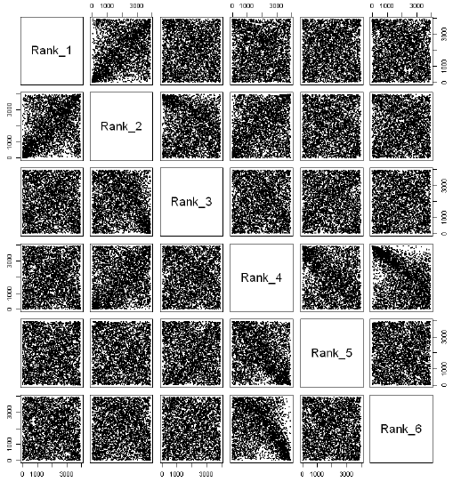
Figure 12 Relationship between SNP rankings of the 6 different SNP sets identified during the hierarchical analysis.

Determination of accuracy of hierarchical panel

Assignment to region has been examined at the different hierarchical scales identified. It has already been shown that it is possible to identify and exclude fish from the NW region from subsequent river level analysis. Table 2 details the accuracy of assignments using the 288 SNP panel at the river level in fish from outwith the NW region using the new baseline and the test assignment files which were assembled ( i.e. the baseline was the full baseline and the assignment mixture file comprised an entire site from each river with two or more sites of data, the Carron, Conon, Dee, Nith, South Esk, Spey and Tweed).

As expected from the regional initial analysis, Table 2 shows that indeed there are very few miss-assignments of fish from the Eastern regions to the NW baseline, and not a single miss-assignment of fish from the Kyle to the ES regions or vice-versa

Table 2 Assignments of fish using the 288 SNP panel examined at the regional level. KY is Kyle, NW is North and West, ES is East and South. Assignments using all data are shown and those using the illustrative assignment score cut-off score of 80.

All data		Assigned origin
	Origin	KY	NW	ES	Correct	% Correct
	KY	58	6	0	58	90.6
	NW	0	0	0	0	N/A
	ES	0	5	229	229	97.9
	% correct	100	N/A	100

All data 80 cut off		Assigned origin
	Origin	KY	NW	ES	Correct	% Correct	% assigned
	KY	56	1	0	56	98.2	89.1
	NW	0	0	0	0	N/A	N/A
	ES	0	4	224	224	98.2	97.4
	% correct	100	N/A	100

Table 3 shows that the Carron fish are seen to have a relatively low assignment success to river, but that the miss-assignments from the Carron are mainly to other rivers in the Kyle region. As all these rivers flow into the same estuary and significant mixing is thought to occur between them, the Kyle rivers were subsequently grouped and successful assignments of the Carron fish examined at this new level as shown in Table 4. As expected, the assignments of these fish are now significantly improved when assigning to this new regional grouping.

Tables 3 and 4 also show that there are relatively low assignment successes in both the Spey and Dee systems. Again these two rivers have been combined and assignment success to the new assignment unit is detailed in Table 5.

Overall, the river level assignments to the combined groups are seen to be very strong ( i.e. ≥ 92.3% accuracy in fish from an assignment group assigning back to that group, Table 5), and considering that the fish being assigned are from sites not represented in the baseline ( i.e. they are not the TS/ HS split data), this suggests that assignments to the river level are likely to be robust where there is sufficient river level SNP coverage to characterise individual rivers well. However, it can be seen that the Dee and Spey are hard to separate in the preceding analysis. It may also be the case that as other rivers are characterised with SNP markers similar patterns might be seen between 2 or more rivers, but at present the extent that this pattern may be manifest is hard to predict.

All data										Assigned origin
Origin	Ayr	Conon	Dee	Dionard	Gruinard	Carron	Cassley	Corriemulzie	Oykel	Shin	Carnoch	Moidart	Helmsdale	Naver	Nesk	Nith	Langadale	Langavat	SEsk	Snizort	Spey	Tay	Tweed	Correct	% Correct
Carron	0	0	0	0	2	7	8	12	2	0	0	0	0	0	0	0	0	0	0	1	0	0	0	7	21.9
Conon	0	25	0	0	0	1	0	2	1	0	0	2	0	0	0	0	0	0	0	1	0	0	0	25	78.1
Dee	0	0	17	0	0	0	0	0	0	0	0	0	0	0	8	0	0	0	0	0	36	0	2	17	27.0
Nith	0	0	0	0	0	0	0	0	0	0	0	1	0	0	0	23	0	0	0	0	3	3	1	23	74.2
SEsk	0	0	1	0	0	0	0	0	0	0	0	0	0	0	0	0	0	0	19	0	2	1	1	19	79.2
Spey	0	0	21	1	0	0	0	0	0	0	0	0	0	0	2	0	0	0	1	1	37	0	1	37	57.8
Tweed	0	0	2	0	0	0	0	0	0	0	0	0	1	0	1	1	0	0	0	1	1	3	42	42	80.8
% Correct		100.0	41.5			87.5										95.8			95.0		46.8		89.4

All data 80 cut off										Assigned origin
Origin	Ayr	Conon	Dee	Dionard	Gruinard	Carron	Cassley	Corriemulzie	Oykel	Shin	Carnoch	Moidart	Helmsdale	Naver	Nesk	Nith	Langadale	Langavat	SEsk	Snizort	Spey	Tay	Tweed	Correct	% Correct	% assigned
Carron	0	0	0	0	0	5	8	7	1	0	0	0	0	0	0	0	0	0	0	0	0	0	0	5	23.8	65.6
Conon	0	23	0	0	0	0	0	2	1	0	0	1	0	0	0	0	0	0	0	0	0	0	0	23	85.2	84.4
Dee	0	0	8	0	0	0	0	0	0	0	0	0	0	0	4	0	0	0	0	0	26	0	0	8	21.1	60.3
Nith	0	0	0	0	0	0	0	0	0	0	0	0	0	0	0	18	0	0	0	0	1	2	1	18	81.8	71.0
SEsk	0	0	0	0	0	0	0	0	0	0	0	0	0	0	0	0	0	0	14	0	0	0	1	14	93.3	62.5
Spey	0	0	13	1	0	0	0	0	0	0	0	0	0	0	2	0	0	0	0	0	24	0	1	24	58.5	64.1
Tweed	0	0	1	0	0	0	0	0	0	0	0	0	0	0	1	0	0	0	0	1	1	0	36	36	90.0	76.9
% Correct		100.0	36.4			100.0										100.0			100.0		46.2		92.3

Table 3 Assignment success using the 288 SNP panel to river level.

All data								Assigned origin
Origin	Ayr	Conon	Dee	Dionard	Gruinard	Kyle	Shin	Carnoch	Moidart	Helmsdale	Naver	Nesk	Nith	Langadale	Langavat	SEsk	Snizort	Spey	Tay	Tweed	Correct	% Correct
Carron	0	0	0	0	2	29	0	0	0	0	0	0	0	0	0	0	1	0	0	0	29	90.6
Conon	0	25	0	0	0	1	0	0	2	0	0	0	0	0	0	0	1	0	0	0	25	78.1
Dee	0	0	17	0	0	0	0	0	0	0	0	8	0	0	0	0	0	36	0	2	17	27.0
Nith	0	0	0	0	0	0	0	0	1	0	0	0	23	0	0	0	0	3	3	1	23	74.2
SEsk	0	0	1	0	0	0	0	0	0	0	0	0	0	0	0	19	0	2	1	1	19	79.2
Spey	0	0	21	1	0	0	0	0	0	0	0	2	0	0	0	1	1	37	0	1	37	57.8
Tweed	0	0	2	0	0	0	0	0	0	1	0	1	1	0	0	0	1	1	3	42	42	80.8
% Correct		100.0	41.5			96.7							95.8			95.0		46.8		89.4

All data 80 cut off								Assigned oigin
Origin	Ayr	Conon	Dee	Dionard	Gruinard	Kyle	Shin	Carnoch	Moidart	Helmsdale	Naver	Nesk	Nith	Langadale	Langavat	SEsk	Snizort	Spey	Tay	Tweed	Correct	% Correct	% assigned
Carron	0	0	0	0	0	21	0	0	0	0	0	0	0	0	0	0	0	0	0	0	21	100.0	65.6
Conon	0	23	0	0	0	0	0	0	1	0	0	0	0	0	0	0	0	0	0	0	23	85.2	84.4
Dee	0	0	8	0	0	0	0	0	0	0	0	4	0	0	0	0	0	26	0	0	8	21.1	60.3
Nith	0	0	0	0	0	0	0	0	0	0	0	0	18	0	0	0	0	1	2	1	18	81.8	71.0
SEsk	0	0	0	0	0	0	0	0	0	0	0	0	0	0	0	14	0	0	0	1	14	93.3	62.5
Spey	0	0	13	1	0	0	0	0	0	0	0	2	0	0	0	0	0	24	0	1	24	58.5	64.1
Tweed	0	0	1	0	0	0	0	0	0	0	0	1	0	0	0	0	1	1	0	36	36	90.0	76.9
% Correct		100.0	36.4			100.0							100.0			100.0		46.2		92.3

Table 4 Assignment success using the 288 SNP panel to river level with the individual Kyle rivers combined.

All data								Assigned origin
Origin	Ayr	Conon	Dee/Spey	Dionard	Gruinard	Kyle	Shin	Carnoch	Moidart	Helmsdale	Naver	Nesk	Nith	Langadale	Langavat	SEsk	Snizort	Tay	Tweed	Correct	% Correct
Carron	0	0	0	0	2	29	0	0	0	0	0	0	0	0	0	0	1	0	0	29	90.6
Conon	0	25	0	0	0	1	0	0	2	0	0	0	0	0	0	0	1	0	0	25	78.1
Dee/Spey	0	0	111	1	0	0	0	0	0	0	0	10	0	0	0	1	1	0	3	111	87.4
Nith	0	0	0	0	0	0	0	0	1	0	0	0	23	0	0	0	0	3	1	23	74.2
SEsk	0	0	1	0	0	0	0	0	0	0	0	0	0	0	0	19	0	1	1	19	79.2
Tweed	0	0	2	0	0	0	0	0	0	1	0	1	1	0	0	0	1	3	42	42	80.8
% Correct		100.0	97.4			96.7							95.8			95.0			89.4

All data 80 cut off								Assigned origin
Origin	Ayr	Conon	Dee/Spey	Dionard	Gruinard	Kyle	Shin	Carnoch	Moidart	Helmsdale	Naver	Nesk	Nith	Langadale	Langavat	SEsk	Snizort	Tay	Tweed	Correct	% Correct	% assigned
Carron	0	0	0	0	0	21	0	0	0	0	0	0	0	0	0	0	0	0	0	21	100.0	65.6
Conon	0	23	0	0	0	0	0	0	1	0	0	0	0	0	0	0	0	0	0	23	85.2	84.4
Dee/Spey	0	0	71	1	0	0	0	0	0	0	0	6	0	0	0	0	0	0	1	71	89.9	62.2
Nith	0	0	0	0	0	0	0	0	0	0	0	0	18	0	0	0	0	2	1	18	81.8	71.0
SEsk	0	0	0	0	0	0	0	0	0	0	0	0	0	0	0	14	0	0	1	14	93.3	62.5
Tweed	0	0	1	0	0	0	0	0	0	0	0	1	0	0	0	0	1	0	36	36	90.0	76.9
% Correct		100.0	98.6			100.0							100.0			100.0			92.3

Table 5 Assignment success using the 288 SNP panel to river level with the individual Kyle rivers combined and also the Spey and Dee combined.

Dee/ Spey separation

A new analysis was performed on just the Dee and Spey data to examine in more detail the possibility of separating Dee and Spey fish. Firstly, relationships between sites in the two rivers was examined using a Neighbour-joining tree ( Saitou and Nei, 1987) and MDS plots using D _A as before. Outlier sites were removed as before and the data were split in half at each site creating a set of individuals to use to rank the SNPs (Training Set, TS) and a set of individuals to test the accuracy of the assignments (Holdout Set, HS). Further, a random site from each river was also completely removed from the TS and added to the HS set. As before, pairwise F _ST was used to rank loci based on their discriminatory power between rivers. Assignments were then performed using different numbers of loci from this ranked list and summing assignment success to the river level.

Three outlier sites are seen when all data is analysed as can be clearly seen on both the tree in Figure 13 and the MDS plot in Figure 14A (Dee Sheeoch, Dee Water Dye, Spey Avon Lyon). When these are removed the two rivers show separation on the Y-axis of the MDS plot in Figure 14B apart from a single Dee site which falls into the Spey grouping on this plot.

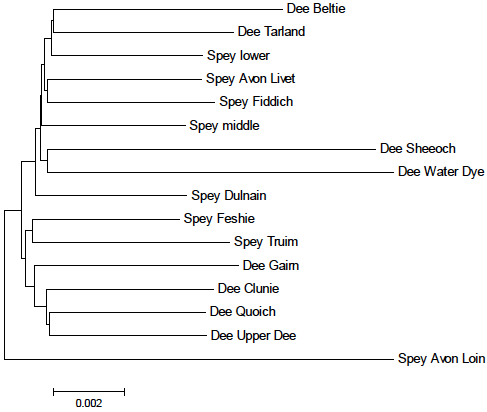
Figure 13 Neighbour-joining tree showing relationships between sites on the Spey and Dee.

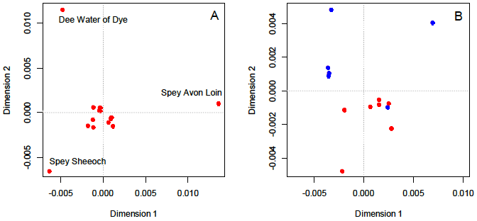
Figure 14 MDS plots of sites pairwise DA between sites on the Spey and Dee. A has all sites and shows the three outliers sites which were removed from the analysis before pairwise DA was recalculated. B shows the relationship between sites with the three outliers removed with Dee sites in blue and Spey in red.

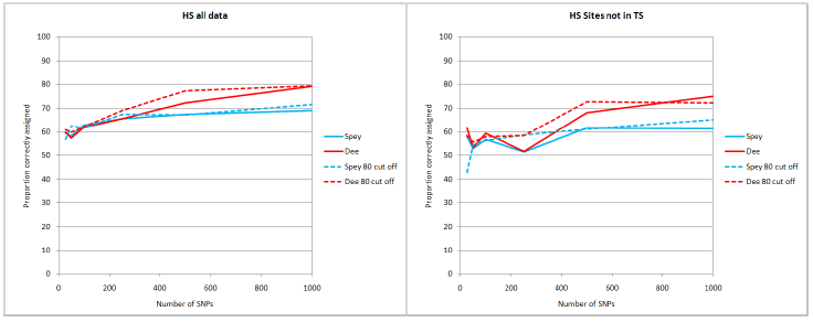
Figure 15 Proportion of fish assigned to a river that are correctly assigned with varying numbers of SNPs. Solid lines are all data dashed are assignments using a cut-off value of 80 for the assignment score.

As before, assignment success of the HS dataset to the TS baseline is shown in Figure 15. Accuracy is seen to be increased compared to the previous analysis (see Table 4). However, the proportion of fish assigning back to a river that actually came from that river is still relatively low (~55 - 80 % of all data and just ~50 - 75 % of sites not in the baseline). By pure chance alone it would be expected that there would be 50% right (two rivers to assign to) and the values are better than this, but not by much until a very large number of SNPs are utilised.

Exclusion of fish from rivers not in the baseline

Exclusion analysis was performed with the aim of removing the fish from rivers not represented in the baseline while at the same time leaving in the assignment of those fish from rivers that were in the baseline. As was hoped it can be seen that the maximum assignment score of fish from rivers not in the baseline is significantly lower than for those fish where their river of origin was present in the baseline ( Figure 16). If a cut-off of 0.05 is used a large proportion of fish from rivers not in the baseline can be removed from the analysis without losing a significant proportion of the other fish.

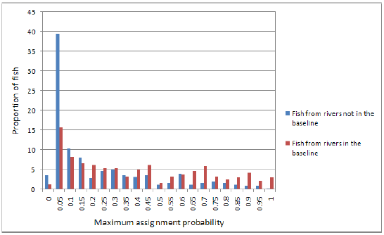
Figure 16 Maximum assignment probabilities of all fish in the analysis.

Variation in the cut-off level of the assignment probability together with variation in the assignment score value cut-off was then examined to determine the optimum level of cut-off for both these metrics where the maximum numbers of fish from rivers not in the baseline are removed while leaving in the analysis those fish from rivers that are represented. As the river level assignments are particularly focused on identifying and assigning fish from the East coast ( i.e. where river level coverage is greatest along with productivity and the presence of Special Areas of Conservation for salmon) the first step in this assignment analysis was to remove any fish that were assigned to the North and West region.

Figure 17 shows the proportion of fish remaining to be assigned after removal of those assigned to the NW region. In this situation, the assignment probability is not yet being used, just removal of all fish assigned to the North and West, which in the mixture file consists of fish from the Helmsdale and Dionard. It can be seen that no matter what the assignment cut-off used, a large proportion of these fish can be removed as they assign to the NW region even though they are from rivers not in the baseline. The regional assignments thus reflect those seen to region in the preceding analysis and are thus very robust.

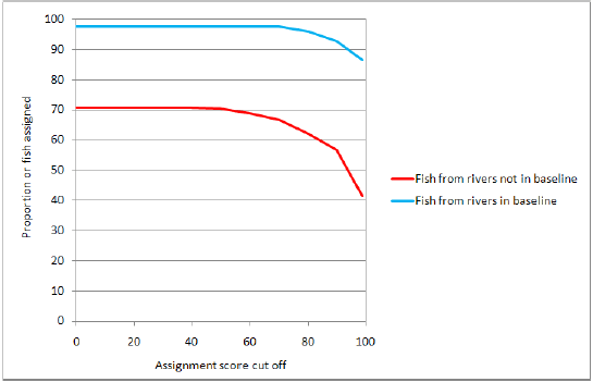
Figure 17 Proportion of fish assigned after removal of fish assigned to the NW region.

The next stage of the exclusion analysis was to utilise the exclusion probability cut-off levels to try to remove the remainder of fish from rivers not represented in the baseline. Different cu-off levels can be used which results in a trade-off between accuracy and numbers of fish remaining in the analysis to be assigned.

As expected by the distribution of assignment probabilities between the two groups of fish, using a cut off probability allows a large proportion of fish from rivers not in the baseline to be removed ( Figure 18). Using an exclusion score of ≤ 0.05, together with an assignment score cut off of 90, is seen to remove ~70 % of fish from rivers not in the baseline while at the same time leaving in ~75 % of fish from rivers represented in the baseline. If a stricter exclusion score of ≤ 0.1 is used together with an assignment score cut off of 90 this is seen to remove ~75 % of fish from rivers not in the baseline while at the same time leaving in ~70 % of fish from rivers represented in the baseline. The lack of significantly greater power to remove more fish from rivers not in the baseline reflects the differential exclusion scores of the two groups of fish as seen in Figure 16. Using a score of 0.05 will remove a much greater proportion of fish from rivers not in the baseline than those in it. However, moving to 0.01, the differential between these two groups is much less and as such the increase in ability to screen out fish from rivers not in the baseline is not increased by a significant amount.

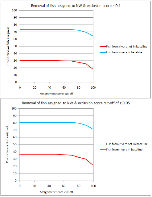
Figure 18 Proportion of fish assigned after removal of fish assigned to the NW region with varying cut-off scores (x-axis) and also utilising the exclusion probabilities of 0.05 and 0.01.

It should also be remembered that in reality the assignment accuracy figures in a real situation might be expected to be better than those reported above. The full baseline will include representation from rivers responsible for the vast majority of production on the East coast. In a realistic mixed stock analysis focusing on this region, the exclusion procedure will be focused on removing fish from outwith the East coast assignment unit. It has been shown that this can be done with accuracy; leaving fish to be assigned within the East coast assignment unit which again has been shown can be (apart from the separation of the Spey/Dee) performed with good accuracy (at least in the rivers analysed so far).

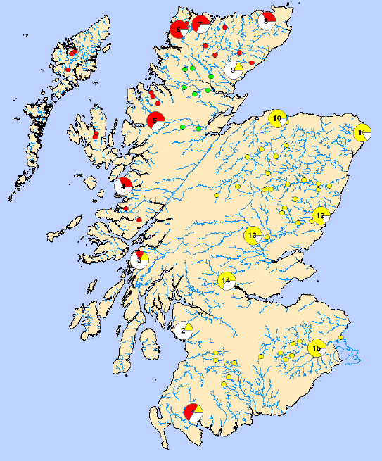
Figure 19 Regional assignment summary of test fish to second level regional assignment units assignments using an assignment confidence cut-off score of 90 and an exclusion probability cut-off of 0.5. Baseline sites are shown as small circles with their colour representing their assignment group: Green are Kyle of Sutherland group ( KY), yellow are east and south group ( ES), red are north and west group ( NW), white are unassigned fish. Pie-charts show the assignments of the test fish. As there were 6 test fish at each site pie-chart segments can be seen to relate to individual fish. 1 River Cree, 2 River Garnock, 3 River Euchar, 4 River Morar, 5 River Ewe, 6 Rhiconich River, 7 River Hope, 8 River Thurso, 9 River Brora, 10 River Lossie, 11 River Ugie, 12 River North Esk, 13 River Tay, 14 River Forth, 15 River Tweed.

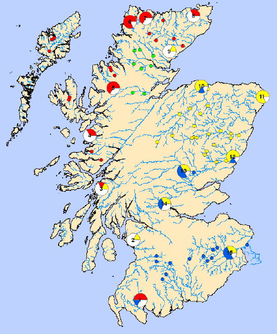
Figure 20 Regional assignment summary of test fish to third level regional assignment units assignments using an assignment confidence cut-off score of 90 and an exclusion probability cut-off of 0.5. Baseline sites are shown as small circles with their colour representing their assignment group: Green are Kyle of Sutherland group ( KY), yellow are east group ( ES), red are north and west group ( NW), blue are south (S) group white are unassigned fish. Pie-charts show the assignments of the test fish. As there were 6 test fish at each site pie-chart segments can be seen to relate to individual fish. 1 River Cree, 2 River Garnock, 3 River Euchar, 4 River Morar, 5 River Ewe, 6 Rhiconich River, 7 River Hope, 8 River Thurso, 9 River Brora, 10 River Lossie, 11 River Ugie, 12 River North Esk, 13 River Tay, 14 River Forth, 15 River Tweed.

Table 6 Assignment proportions of fish in the regional test panel to second and third level assignment regions as depicted in Figures 19 and 20. Assignment units are: Kyle of Sutherland group ( KY), East and South group ( ES), North and West group ( NW), East group, (E) and South group (S). Non-Ass refers to non-assigned fish after the cut-off has been applied (see text).

Site code	River	Second level regions				Third level regions
		ES	KY	NW	Non-Ass	E	S	KY	NW	Non-Ass
1	River Cree	83.3	0.0	0.0	16.7	33.3	50.0	0.0	0.0	16.7
2	River Garnock	16.7	0.0	16.7	66.7	16.7	0.0	0.0	16.7	66.7
3	River Euchar	83.3	0.0	0.0	16.7	83.3	0.0	0.0	0.0	16.7
4	River Morar	66.7	0.0	0.0	33.3	33.3	33.3	0.0	0.0	33.3
5	River Ewe	16.7	0.0	0.0	83.3	16.7	0.0	0.0	0.0	83.3
6	Rhiconich River	83.3	0.0	0.0	16.7	66.7	16.7	0.0	0.0	16.7
7	River Hope	83.3	0.0	0.0	16.7	33.3	50.0	0.0	0.0	16.7
8	River Thurso	16.7	0.0	0.0	83.3	16.7	0.0	0.0	0.0	83.3
9	River Brora	16.7	0.0	50.0	33.3	0.0	16.7	0.0	50.0	33.3
10	River Lossie	0.0	0.0	33.3	66.7	0.0	0.0	0.0	33.3	66.7
11	River Ugie	0.0	0.0	83.3	16.7	0.0	0.0	0.0	83.3	16.7
12	River North Esk	0.0	0.0	33.3	66.7	0.0	0.0	0.0	33.3	66.7
13	River Tay	83.3	0.0	0.0	16.7	66.7	16.7	0.0	0.0	16.7
14	River Forth	0.0	0.0	66.7	33.3	0.0	0.0	0.0	66.7	33.3
15	River Tweed	0.0	0.0	66.7	33.3	0.0	0.0	0.0	66.7	33.3

Regional assignment test

Assignments of the fish used in the regional assignment test using an assignment confidence cut-off score of 90 and an exclusion probability cut-off of 0.5 are detailed in Figures 19 and 20 and Table 6. Figure 19 shows all top assignments for all fish to the three regional groups at the second regional level examined. In general the assignments are very accurate with fish from the ES unit mostly being correctly identified as coming from the region and fish from the NW from that region. There are 4 miss-assigned fish in the NW/ KY regions which are assigning to the ES group.

Examination of the second regional level of assignment in Figure 20 shows interesting patterns of assignment. Firstly, NW fish are being assigned to the NW with none being miss-assigned to this group from the E region. Within what was previously the ES region though, there is some mixing of assignments to the E and S units in many of the sites. There is also a number of fish in the west coast of the S unit (from the river Cree) which do not assign to the S unit but rather the NW unit. In general, the S unit is poorly characterised in the baseline available here. South of the Esks there is just a single site on the Tay and the nothing else between the Tay and the Tweed. Further, within the S unit the Tweed is well characterised, but the western coast rivers which have been characterised as being within this unit have only sites from the far upper sections of their catchments. When a site from the lower catchment has been included on the Cree, it can be seen that the majority of fish from their assign to the NW rather than the S group. These observations suggest that the S group is not well characterised. The upper sites on the west coast rivers that have been included in the S group may not actually be representative of the majority of the main river stocks on the west coast in the S region, which may actually group with the rest of the NW assignment unit. With the baseline used to define the region groups at this level the upper sites may have grouped with the Tweed as there was little else around the southern part of the west coast for them to group with. Better characterisation of rivers from the Clyde and south to the Scottish boarder would help resolve this picture and it might be expected that the sites in on the west coast of what has been characterised here as the S unit might resolve into a well-defined South West grouping.

Similarly, on the southern part of the east coast grouping, the surprising fact that the single site on the Tay grouped with the Tweed could again be reflective of poor and unrepresentative coverage of fish from this part of the region within this assignment unit. More samples are needed from the Tay, Earn and Forth catchments to resolve this picture better. The patterns of assignment of fish from the test panel within this region might then be expected to be better explained.

It should also be remembered that these results come from an analysis using just 89 SNP markers, and when the full set of 288 is employed it would be expected that the accuracy and confidence of the assignments will likely increase.