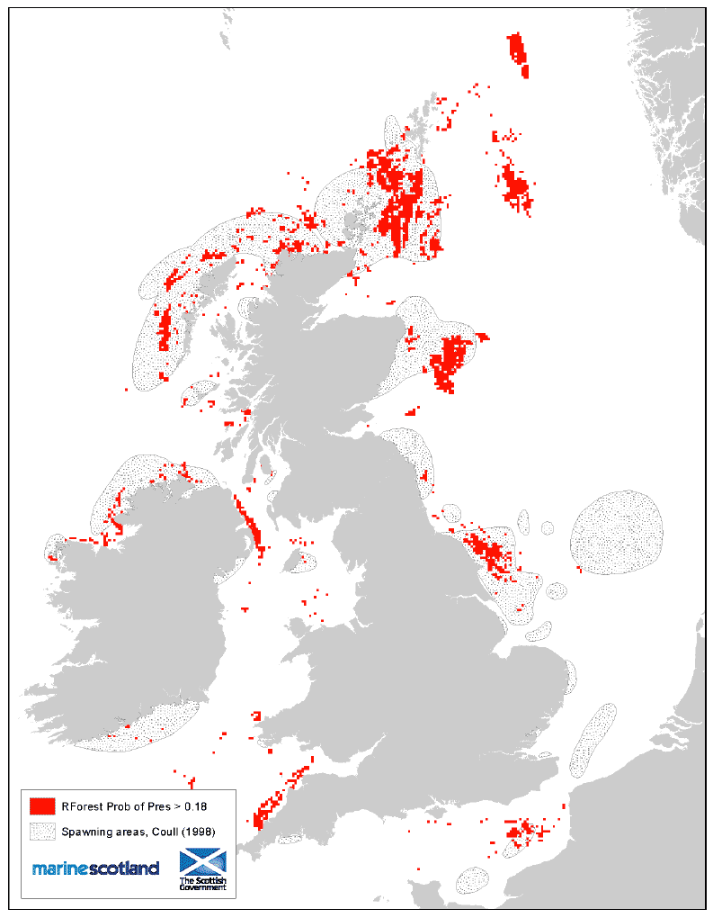
Scottish Marine and Freshwater Science Volume 5 Number 10: Updating Fisheries Sensitivity Maps in British Waters

3 Fisheries Sensitivity Maps

3.1 Areas of 0 Group Aggregations

There is a set of three maps for each of the selected species:

a) The first map shows the probability of presence of aggregations of 0 group fish; aggregations were determined as detailed in Section 2.1.1. For hake and anglerfish the maps presented here show the probability of presence of 0 group fish and not the probability of presence of aggregations.

The first map also shows information about the performance of the Random Forest model, evaluated by the AUC and kappa statistics, as explained in Section 2.3. Random Forest always showed higher values than MAXENT and, therefore, this model was used to produce the final outputs.
A summary of the performance of every model can be seen in Table 7 and Table 8.

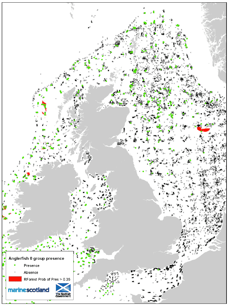
b) The second map shows areas of 0 group aggregations in red, identified as the areas with a probability of presence above the value at which kappa is maximum - as detailed in Section 2.3

This map also shows Presence and Absence source data.

c) The third map shows how the newly defined 0 group aggregation areas compare to the areas defined in Coull et al. (1998), for the species where these were available. Horse mackerel, hake and anglerfish were not included in the Coull (1998) report hence for these three species there are no maps of this kind.

Table 7

Evaluation of models performance: AUC (Area Under the Curve) and kappa statistics, using a random division of the data.

	AUC		Kappa
	Value	Performance	Value	Performance
Cod	0.977 ± 0.018	Excellent	0.682 ± 0.053	Good
Haddock	0.987 ± 0.009	Excellent	0.859 ± 0.043	Excellent
Whiting	0.980 ± 0.005	Excellent	0.823 ± 0.021	Excellent
Norway pout	0.988 ± 0.005	Excellent	0.861 ± 0.023	Excellent
Herring	0.949 ± 0.012	Excellent	0.539 ± 0.033	Good
Mackerel	0.985 ± 0.010	Excellent	0.837 ± 0.057	Excellent
Horse mackerel	0.988 ± 0.004	Excellent	0.848 ± 0.033	Excellent
Sprat	0.988 ± 0.010	Excellent	0.857 ± 0.049	Excellent
Blue whiting	0.997 ± 0.002	Excellent	0.879 ± 0.038	Excellent
Plaice	0.997 ± 0.003	Excellent	0.893 ± 0.030	Excellent
Sole	0.995 ± 0.007	Excellent	0.750 ± 0.096	Excellent
Hake	0.977 ± 0.005	Excellent	0.657 ± 0.034	Good
Anglerfish	0.979 ± 0.013	Excellent	0.667 ± 0.036	Good

Table 8

Evaluation of models performance: AUC (Area Under the Curve) and kappa statistics, using a year-by-year division of the data.

Herring, mackerel and sole were not analysed using this division of data.

	AUC		Kappa
	Value	Performance	Value	Performance
Cod	0.79 ± 0.08	Good	0.19 ± 0.08	Poor
Haddock	0.82 ± 0.08	Good	0.37 ± 0.07	Poor
Whiting	0.83 ± 0.05	Good	0.42 ± 0.08	Good
Norway pout	0.86 ± 0.04	Good	0.38 ± 0.1	Poor
Herring	-	-	-	-
Mackerel	-	-	-	-
Horse mackerel	0.91 ± 0.07	Excellent	0.51 ± 0.15	Good
Sprat	0.86 ± 0.08	Good	0.33 ± 0.11	Poor
Blue whiting	0.95 ± 0.03	Excellent	0.51 ± 0.18	Good
Plaice	0.96 ±0.03	Excellent	0.67 ± 0.16	Good
Sole	-	-	-	-
Hake	0.92 ± 0.05	Excellent	0.47 ± 0.17	Good
Anglerfish	0.97 ± 0.01	Excellent	0.67 ± 0.03	Good

Figure 3: Probability of presence of 0 group aggregations. Cod.

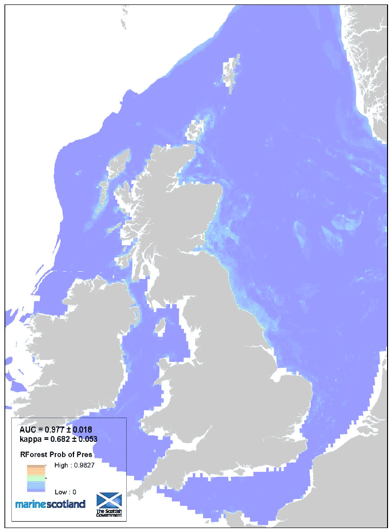
Figure 4: 0 group aggregations and areas of Presence/Absence source data. Cod.

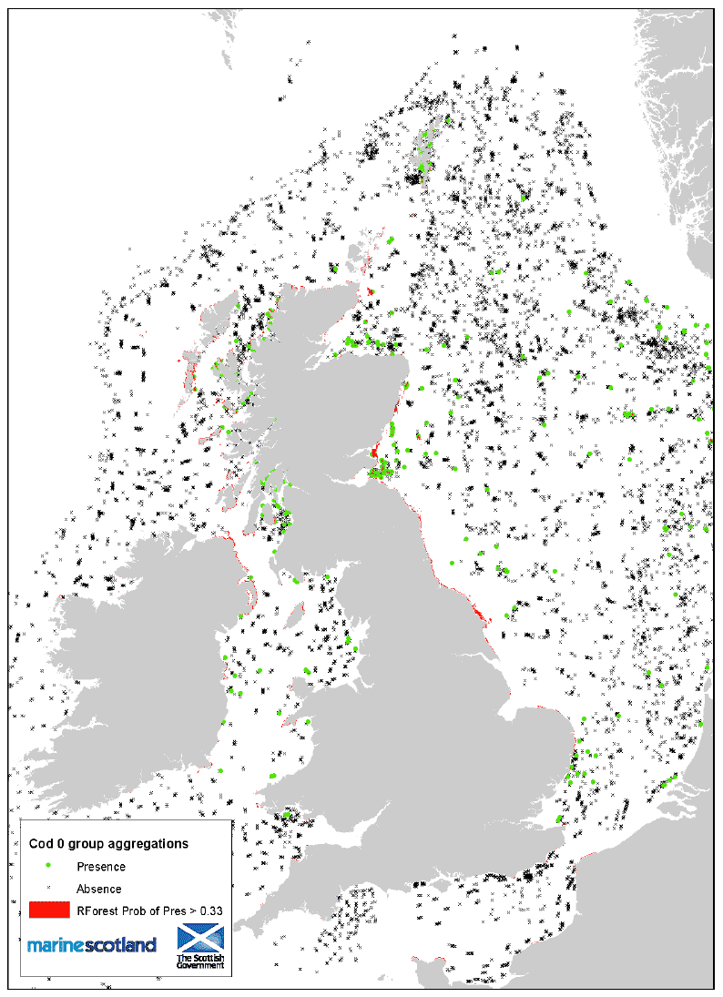
Figure 5: 0 group aggregation areas and Coull (1998) nursery areas. Cod.

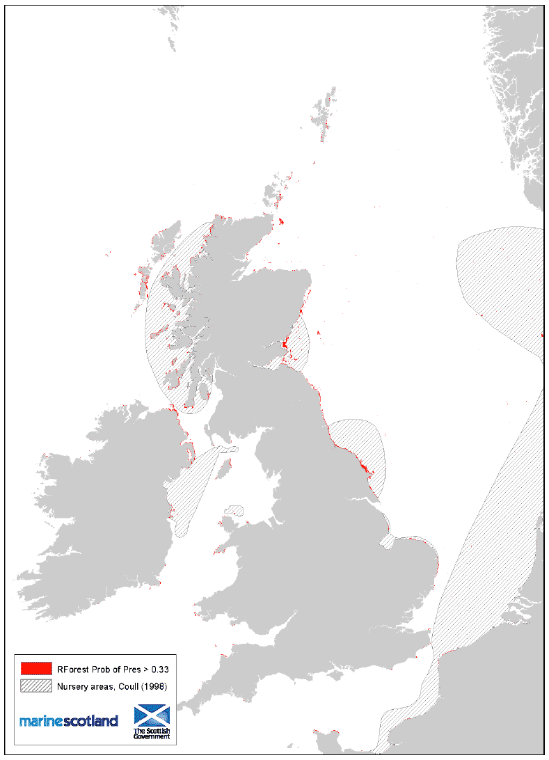
Figure 6: Probability of presence of 0 group aggregations. Haddock

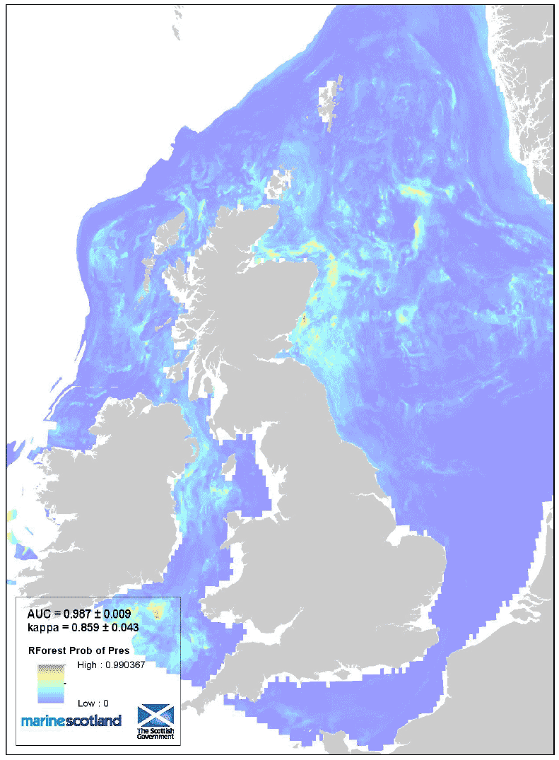
Figure 7: 0 group aggregations and areas of Presence/Absence source data. Haddock.

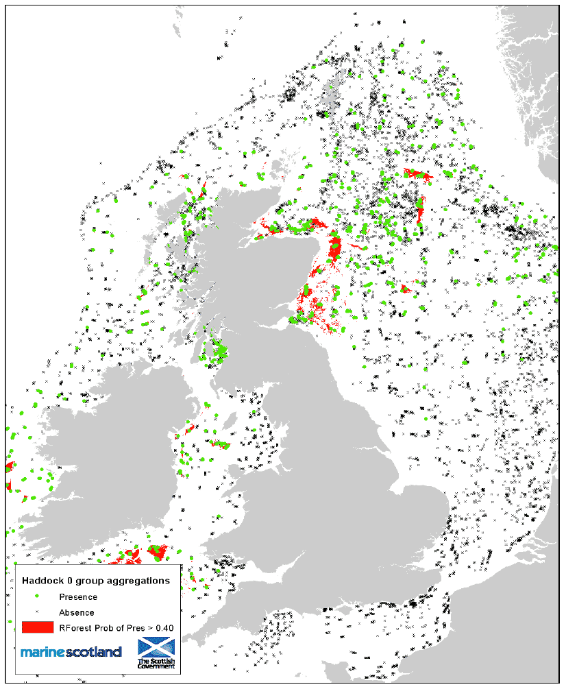
Figure 8: 0 group aggregation areas and Coull (1998) nursery areas. Haddock.

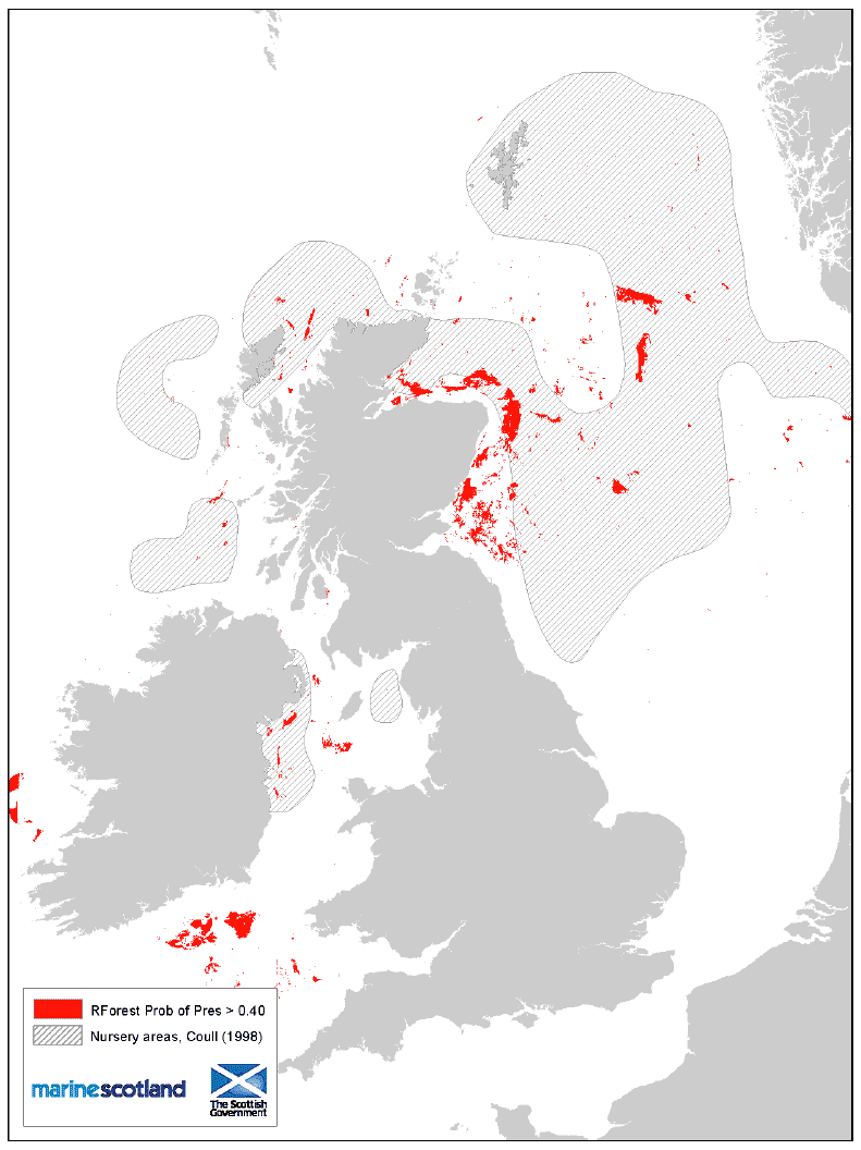
Figure 9: Probability of presence of 0 group aggregations. Whiting.

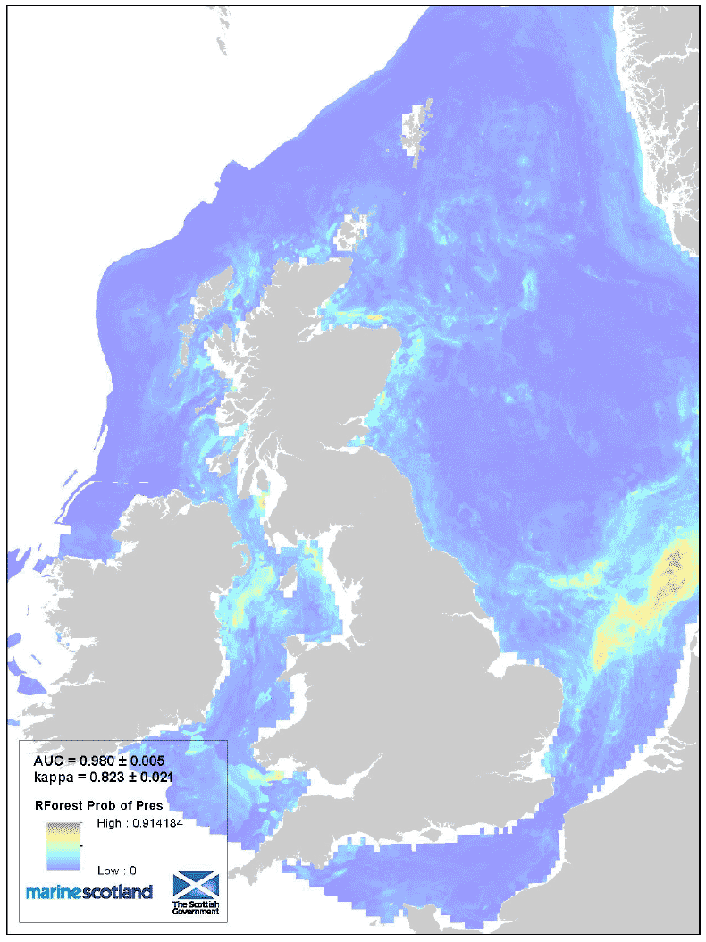
Figure 10: 0 group aggregations and areas of Presence/Absence source data. Whiting.

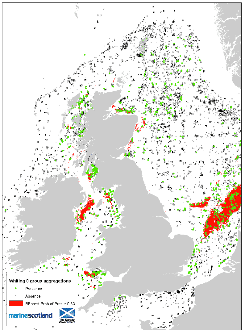
Figure 11: 0 group aggregation areas and Coull (1998) nursery areas. Whiting.

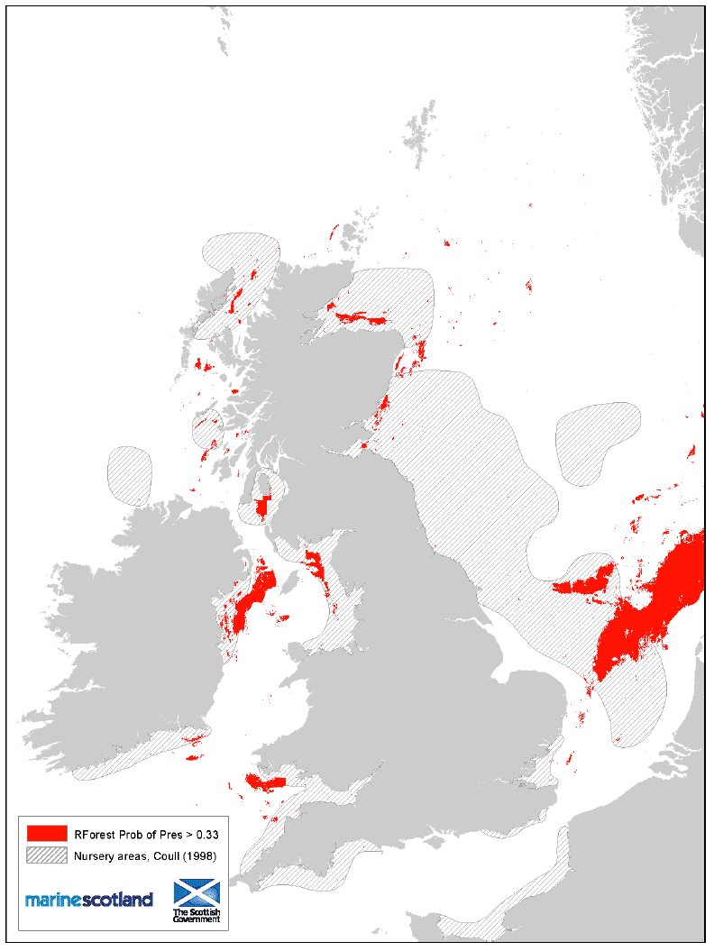
Figure 12: Probability of presence of 0 group aggregations. Norway pout.

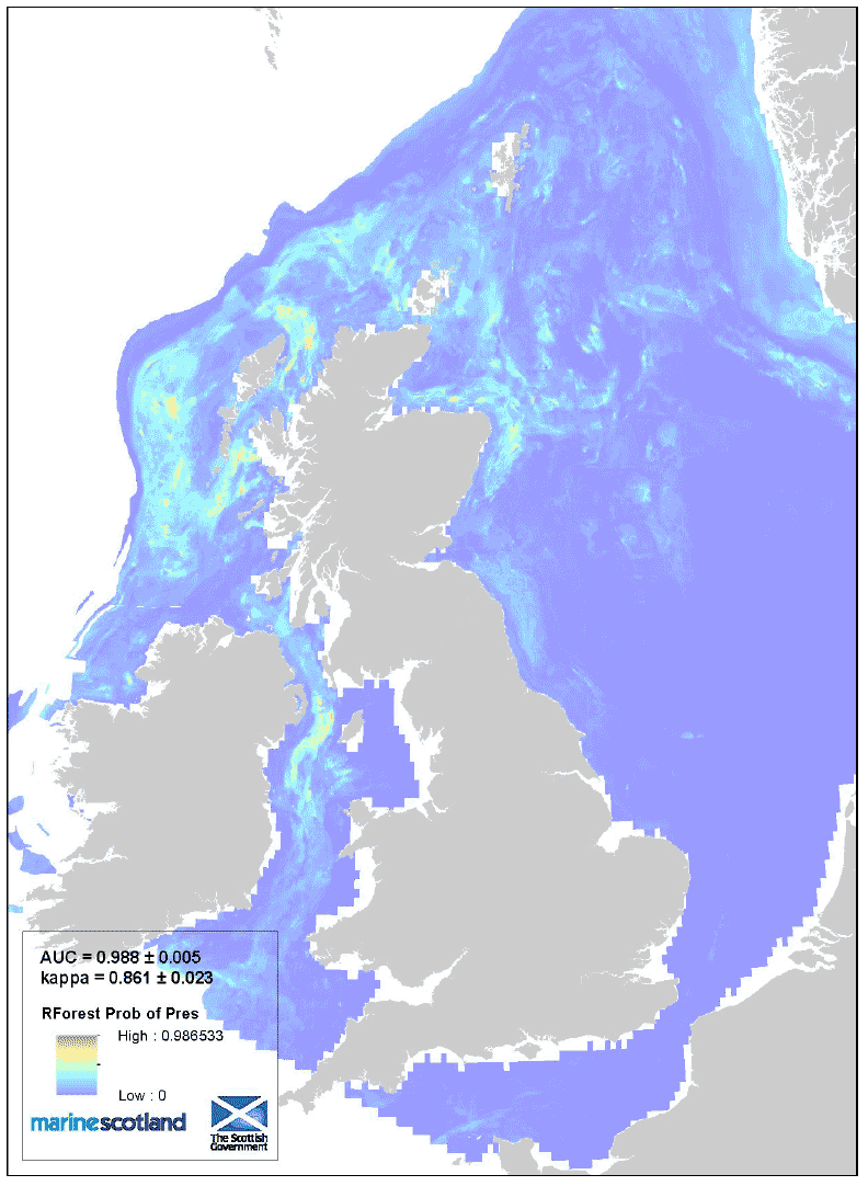
Figure 13: 0 group aggregations and areas of Presence/Absence source data. Norway pout.

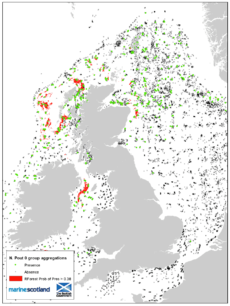
Figure 14: 0 group aggregation areas and Coull (1998) nursery areas. Norway pout.

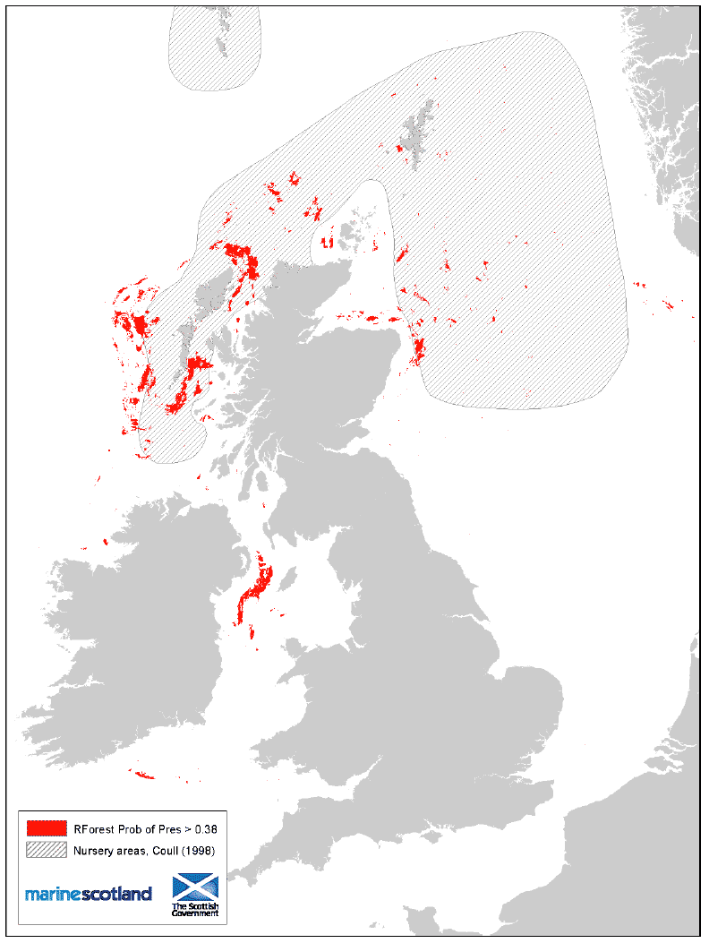
Figure 15: Probability of presence of 0 group aggregations. Herring.

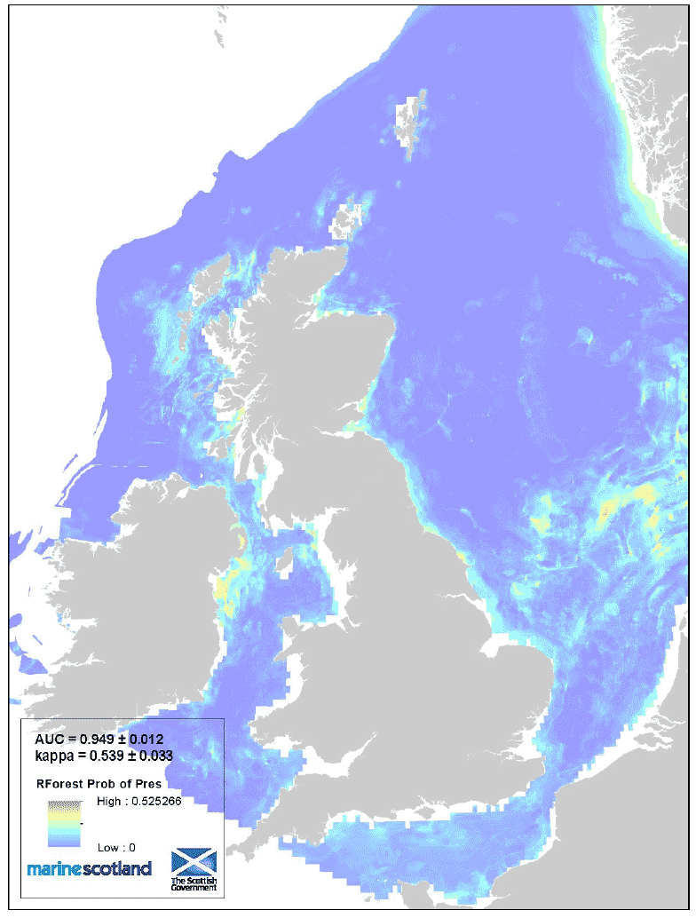
Figure 16: 0 group aggregations and areas of Presence/Absence source data. Herring.

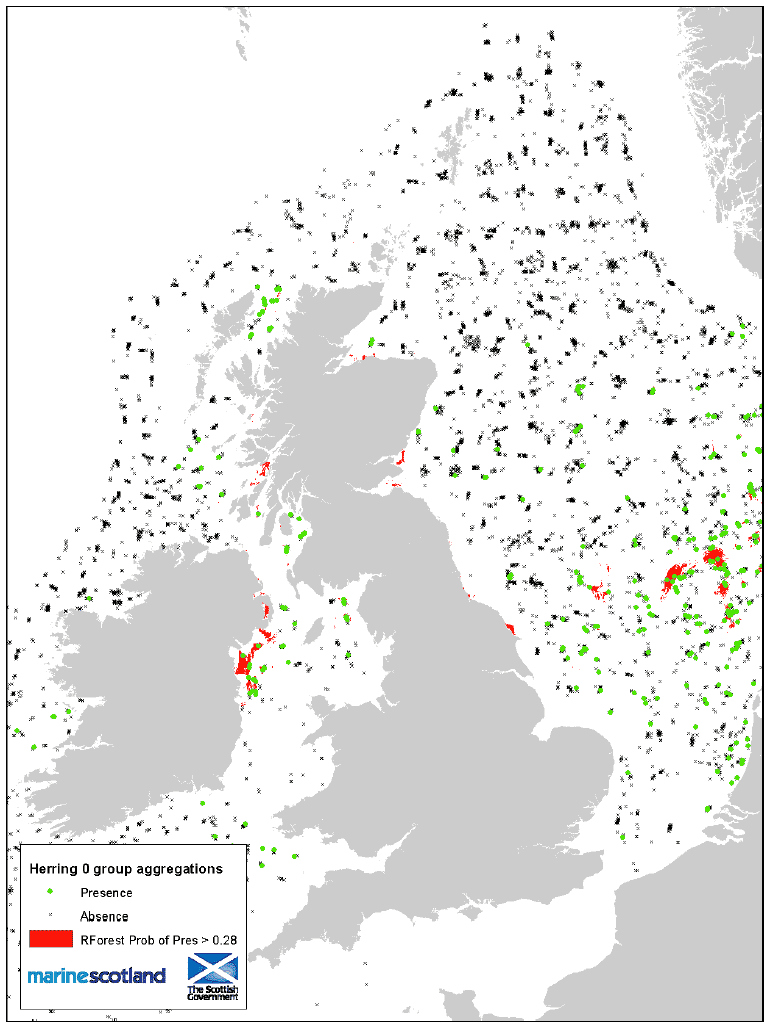
Figure 17: 0 group aggregation areas and Coull (1998) nursery areas. Herring.

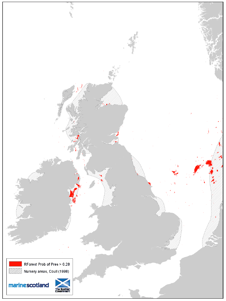
Figure 18: Probability of presence of 0 group aggregations. Mackerel.

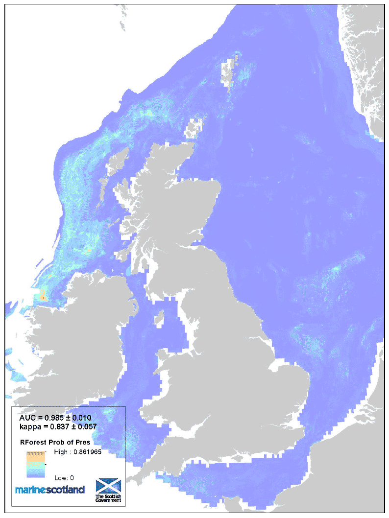
Figure 19: 0 group aggregations and areas of Presence/Absence source data. Mackerel.

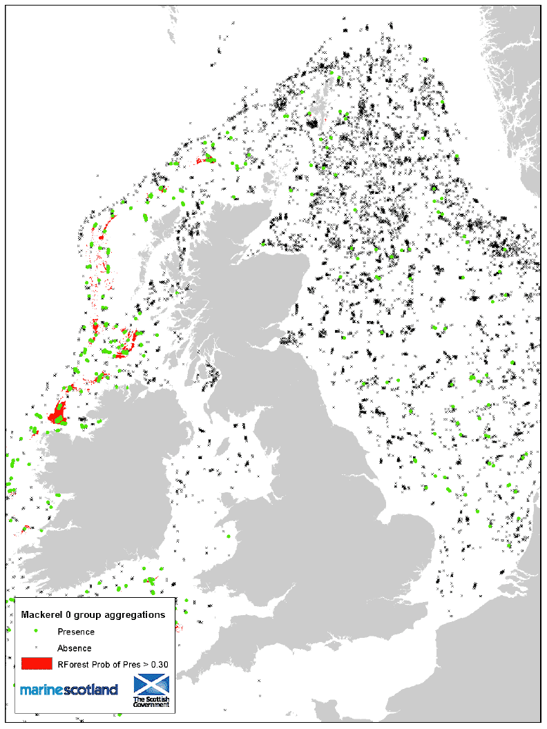
Figure 20: 0 group aggregation areas and Coull (1998) nursery areas. Mackerel.

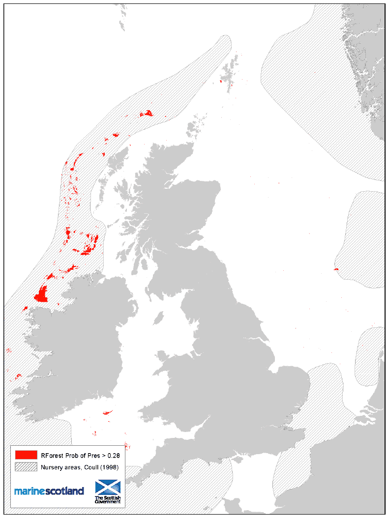
Figure 21: Probability of presence of 0 group aggregations. Horse mackerel.

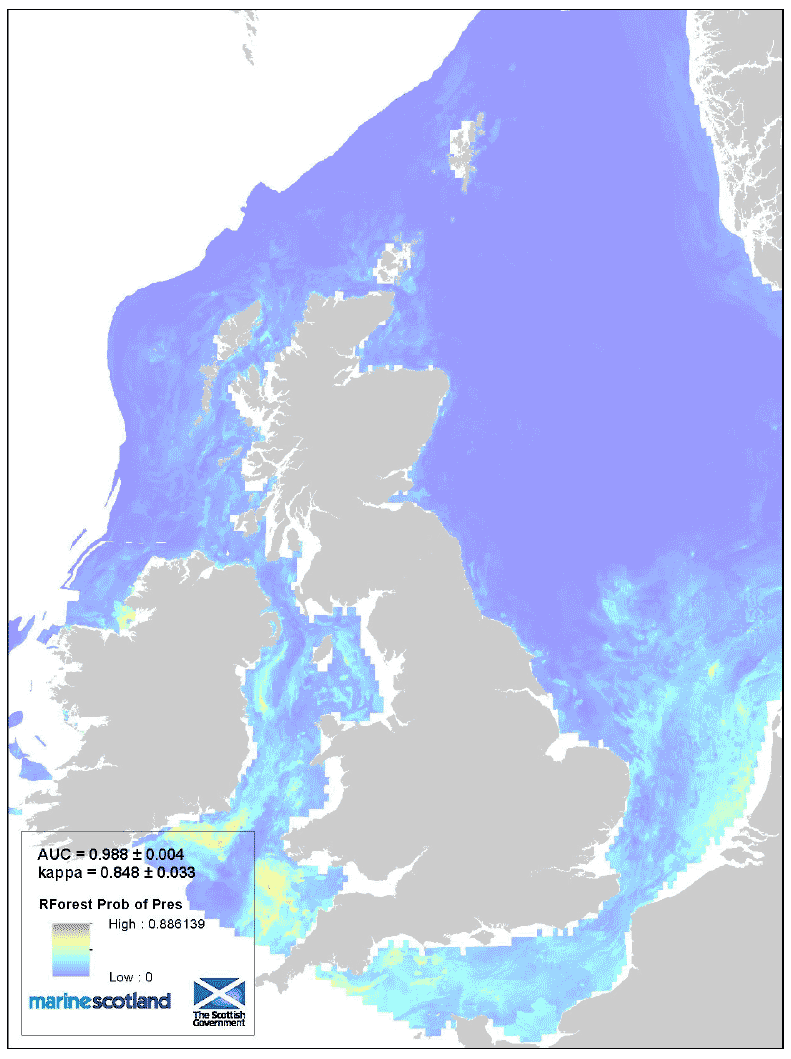
Figure 22: 0 group aggregations and areas of Presence/Absence source data. Horse mackerel.

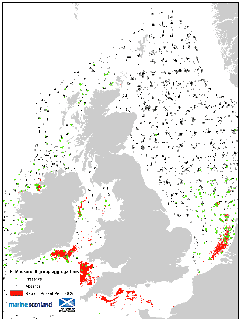
Figure 23: Probability of presence of 0 group aggregations. Sprat.

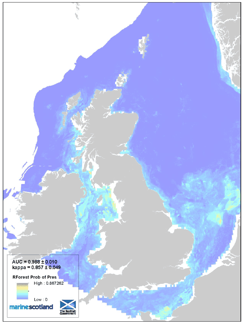
Figure 24: 0 group aggregations and areas of Presence/Absence source data. Horse mackerel.

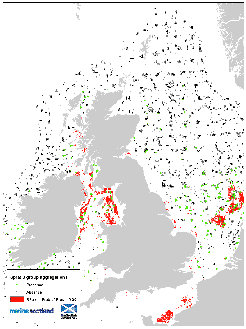
Figure 25: 0 group aggregation areas and Coull (1998) nursery areas. Sprat.

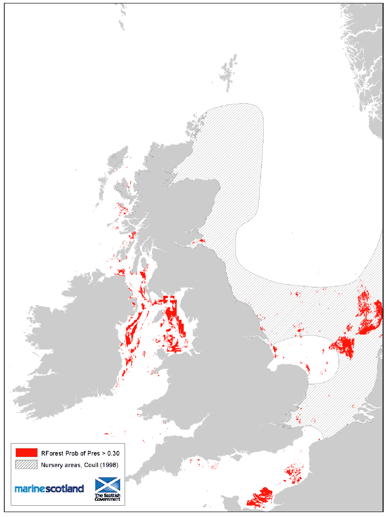
Figure 26: Probability of presence of 0 group aggregations. Blue whiting.

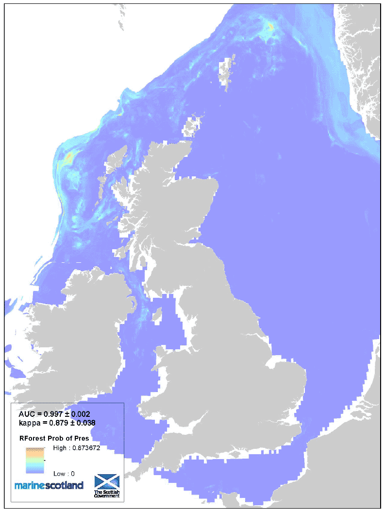
Figure 27: 0 group aggregations and areas of Presence/Absence source data. Blue whiting.

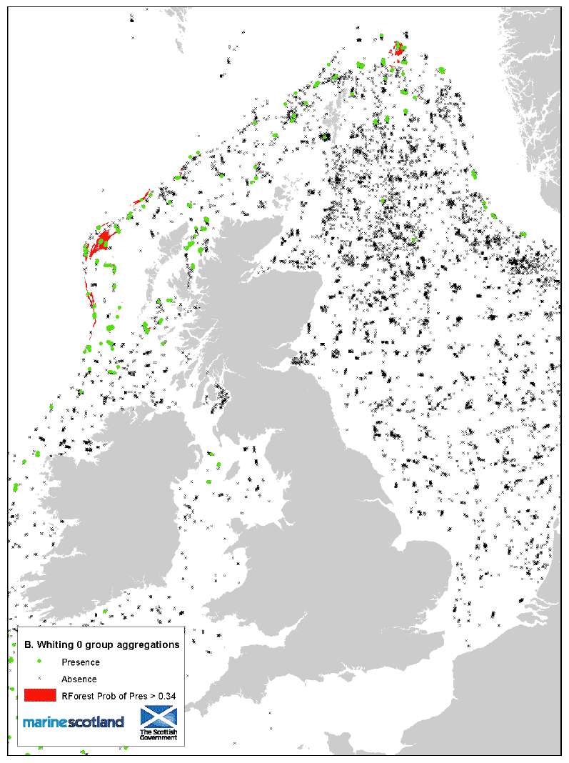
Figure 28: 0 group aggregation areas and Coull (1998) nursery areas. Blue whiting.

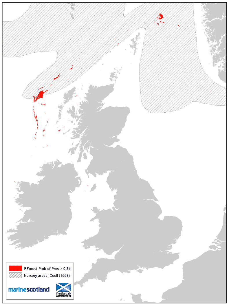
Figure 29: Probability of presence of 0 group aggregations. Plaice.

Figure 30: 0 group aggregations and areas of Presence/Absence source data. Plaice.

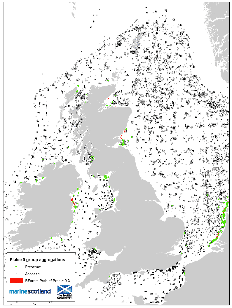
Figure 31: 0 group aggregation areas and Coull (1998) nursery areas. Plaice.

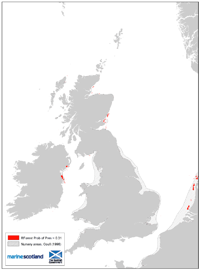
Figure 32: Probability of presence of 0 group aggregations. Sole.

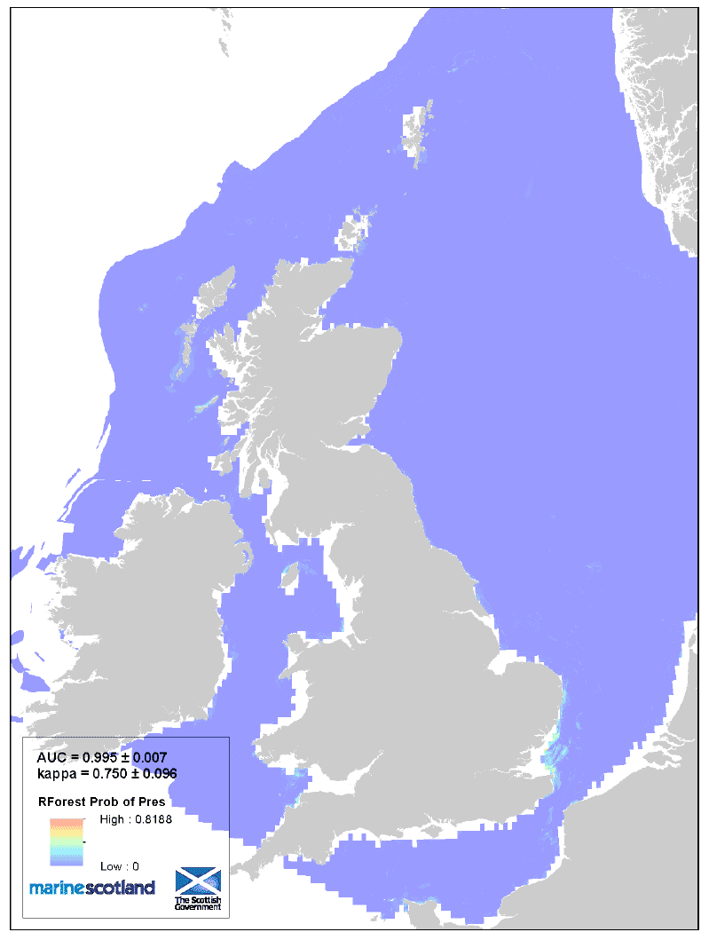
Figure 33: 0 group aggregations and areas of Presence/Absence source data. Sole.

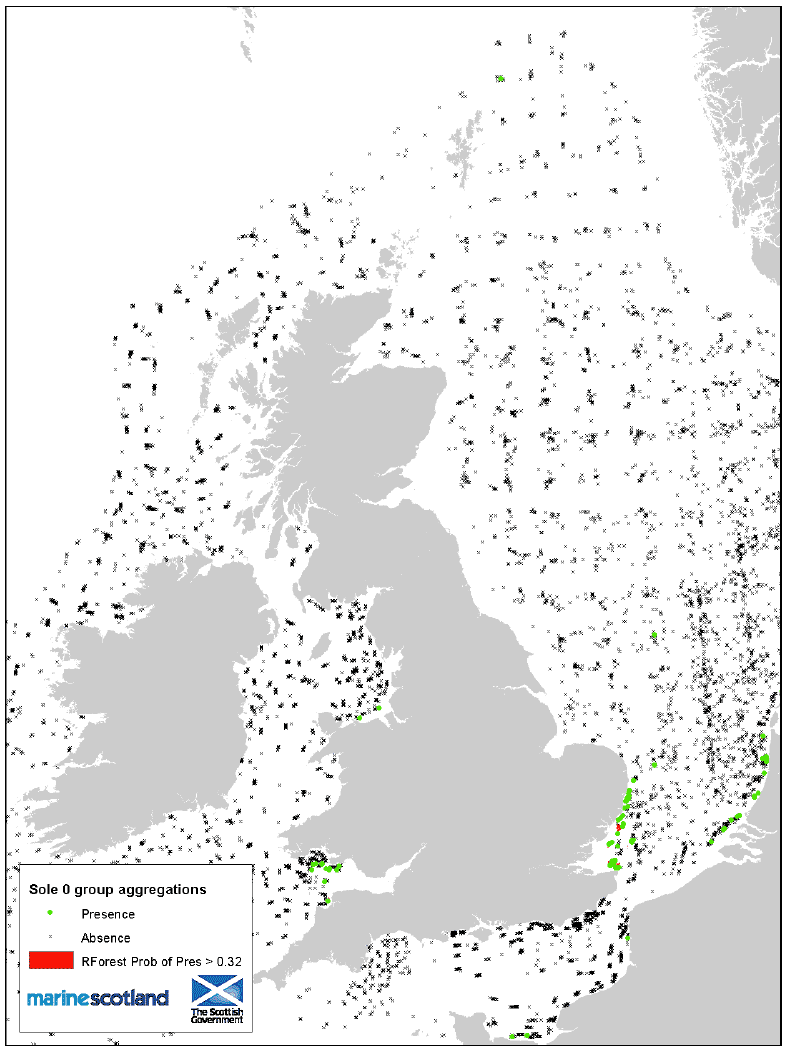
Figure 34: 0 group aggregation areas and Coull (1998) nursery areas. Sole.

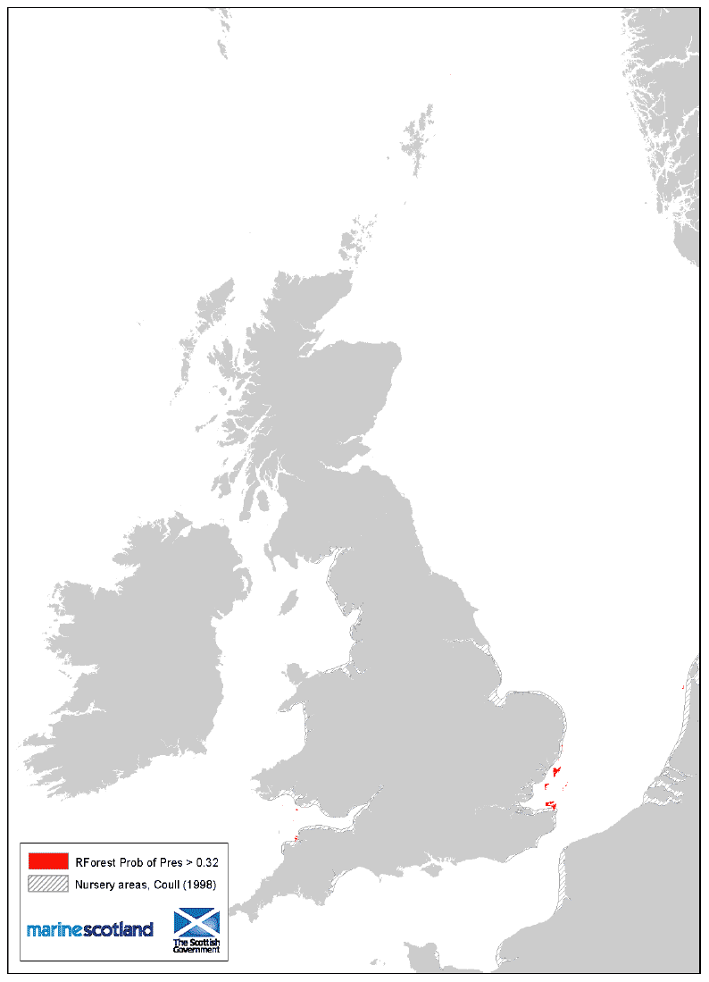
Figure 35: Probability of 0 group presences. Hake.

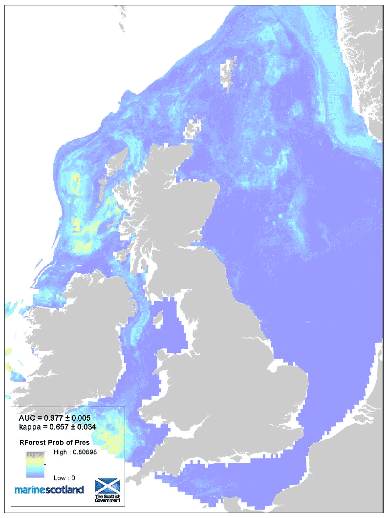
Figure 36: 0 group presence areas and Presence/Absence source data. Hake.

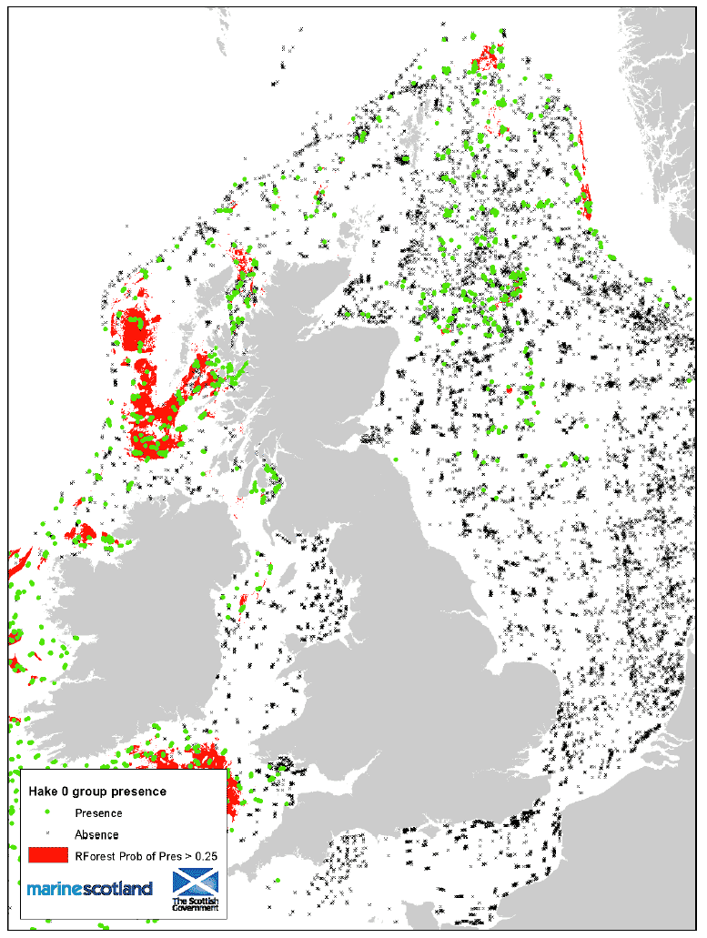
Figure 37: Probability of 0 group presences. Anglerfish.

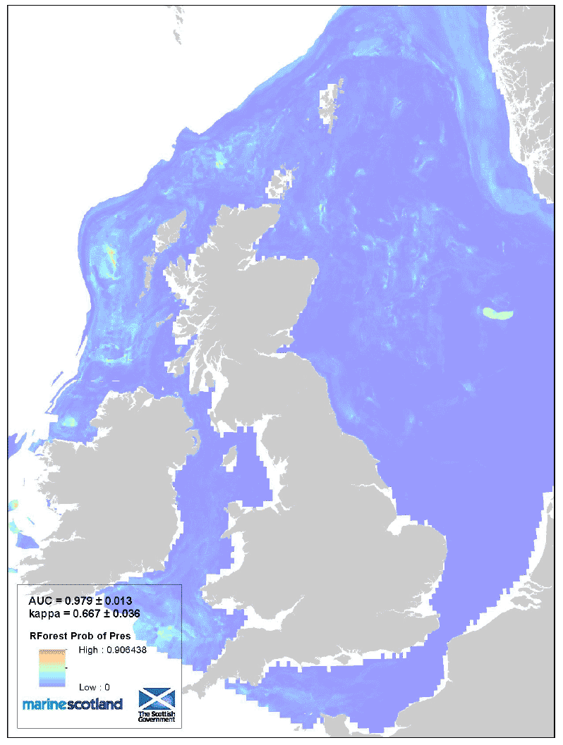
Figure 38: 0 group presence areas and Presence/Absence source data. Anglerfish

3.2 Herring Small Larvae Aggregation Areas

A set of three maps has been created for each of the models, MAXENT and Random Forest:

a) The first map shows the probability of presence of aggregations of small
(<10 mm or <11 mm) herring larvae; aggregations were determined as detailed in Section 2.1.2.

The first map also shows information about the performance of the model, evaluated by the AUC and kappa statistics, as explained in Section 2.3. A summary of the performance of every model can be seen in Table 8.

b) The second map shows areas with high density of small herring larvae, identified as the areas with a probability of presence above the value at which kappa is maximum - as detailed in Section 2.3.

This map also shows Presence and Absence source data.

c) The third map shows how the newly defined areas of small larvae aggregation for herring compare to the spawning areas defined in Coull et al. (1998).

As it has also been explained in Section 2.1.2, two separate and independent runs of the models were done for data east and west of the 4°W meridian.

Table 9

Evaluation of models performance: AUC (Area Under the Curve) and kappa statistics.

	AUC		Kappa
	Value	Performance	Value	Performance
MAXENT - East	0.763 ± 0.017	Good	0.132 ± 0.027	Poor
MAXENT - West	0.762 ± 0.015	Good	0.151 ± 0.027	Poor
RForest - East	0.877 ± 0.009	Good	0.297 ± 0.023	Poor
RForest - West	0.879 ± 0.014	Good	0.319 ± 0.044	Poor

Figure 39: Probability of presence of small larvae aggregations - MAXENT.

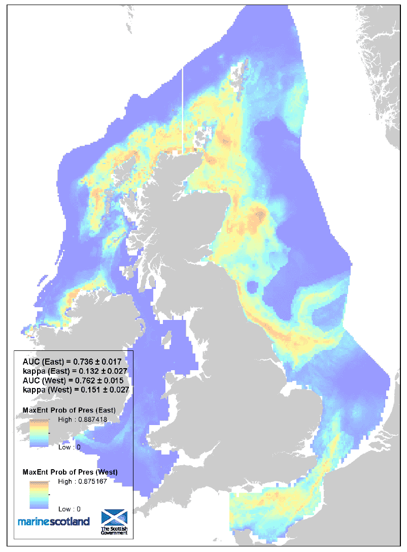
Figure 40: Small larvae aggregation area ( MAXENT) and Presence/Absence source data.

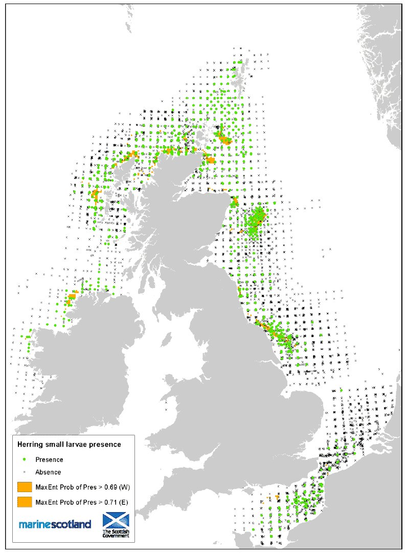
Figure 41: Small larvae aggregation areas ( MAXENT) and Coull spawning areas.

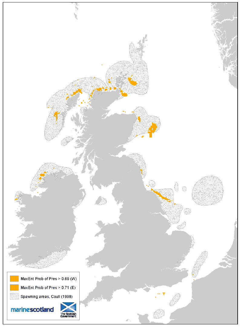
Figure 42: Probability of presence of small larvae aggregations - Random Forest.

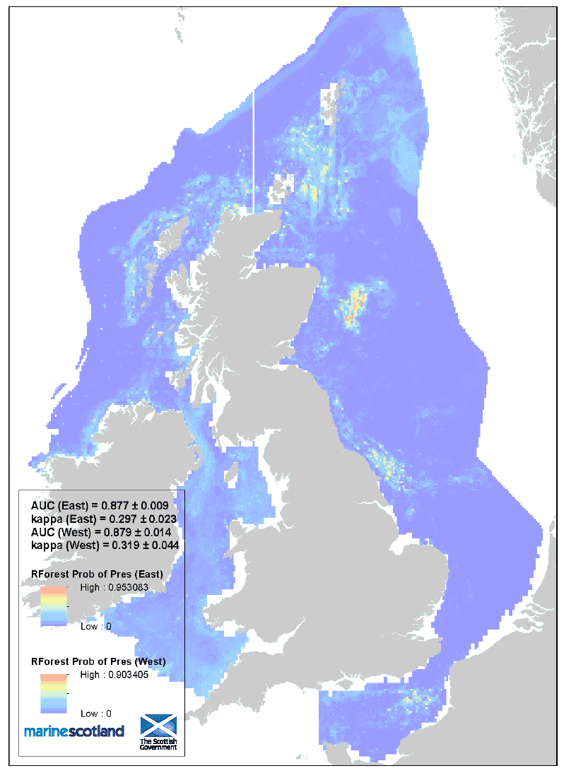
Figure 43: Small larvae aggregation area (Random Forest) and Presence/Absence source data.

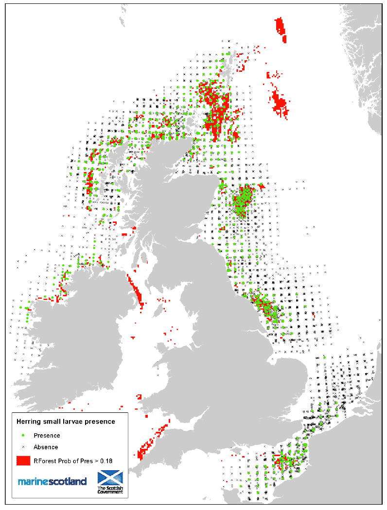
Figure 44: Small larvae aggregation areas (Random Forest) and Coull spawning areas.