Scottish Marine and Freshwater Science Vol 6 No 15: Spatial dynamics of scallops in relation to the Orkney dive fishery. Report of Fishing Industry Science Alliance (FISA) Project 03/12

Methods

Depletion Fishing Experiments

Depletion fishing experiments were undertaken to estimate the density and size-composition of scallop populations at a local scale. Depletion fishing involves repeated removal of catch on a defined sample plot, measuring the rate at which the catch rate declines as the total catch accumulates.

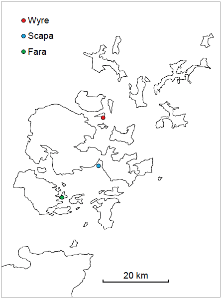
Fifteen depletion experiments were conducted in Orkney waters during 2013 and 2014, comprising five fishing occasions at a location to the south of Wyre, five in Scapa Bay and five close to Fara (Figure 1). The results of the Wyre experiments are reported here, undertaken on board the fishing vessel Three Boys (K905, skipper Emlyn Grieve) at a location to the south of the island (59°6.48'N, 2°57.93W). The survey line was marked out by a heavy sinking rope, left in situ between fishing occasions. Fishing covered a strip of 2 m either side of the rope, and the length of rope covered (and marked for future reference) was 178 m, determined by the coverage of the first bout of fishing. The survey area was thus 712 m ². Fishing was undertaken by a team of four divers employing their usual hand-gathering technique but collecting all sizes of scallops encountered. All scallops captured on each bout of fishing were counted and measured (shell height and width). All scallops not retained for landing were returned to the survey area, distributed along the line by a diver placing scallops on the sea bed. Three fishing bouts were completed on each occasion, limited by dive time and diminishing catch rates. The five depletion fishing occasions were 25 June, 8 August, 7 October and 18 November 2013, and 13 June 2014. Other than the depletion experiments, no fishing activity is thought to have occurred on the Wyre grounds over the duration of the survey series.

Figure 1: Locations of depletion fishing plots in Orkney waters during 2013 and 2014.

Depletion Modelling

Modelling of the changes in catch rate measured over the course of a depletion experiment allows estimation of capture probabilities for a unit of fishing effort and hence of the size of the population from which the catch was drawn. Traditionally this is accomplished using a simple method developed by Leslie and Davis (1939), based on regression of catch rates on cumulative catch. A statistically more rigorous maximum likelihood approach has been developed for the analysis of data from these experiments, allowing likelihood-based inferences about parameter uncertainty and variability of capture probabilities between size-groups and survey occasions. Population estimates and capture probabilities were constrained within feasible bounds by log - and logistic transformation respectively. Five models were considered for variation in capture probability between size-groups and survey occasions:

(i) time * size, in which separate capture probabilities are estimated for each size-group and survey occasion independently - this is equivalent to fitting a separate model to the data for each size-group on each occasion;

(ii) time + size, in which the effects of size-group and survey occasion on capture probability are additive on a logistic scale - this means that differences among size-groups are modelled as being consistent between survey occasions (or, equivalently, that differences among survey occasions are consistent between size-groups);

(iii) time, in which capture probabilities are modelled as differing between survey occasions but the same in all size-groups;

(iv) size, in which capture probabilities are modelled as differing between size- groups but the same on all survey occasions; and

(v) constant, in which capture probabilities are modelled as being the same on all survey occasions and in all size-groups.

Population numbers were treated as free parameters in all models, being the outcome of catch scaled by capture probability. The simplest adequate model for the data was selected by minimum value of the Akaike Information Criterion, adjusted for small sample size according to Burnham & Anderson (2002). Catch numbers, being count data, were modelled as Poisson distributed. Overdispersion in the count data was accounted for by estimating a dispersion coefficient ( c, variance inflation factor) based on the Pearson _X ² statistic for the full size * time model:

, Eq. 1

where df is the degrees of freedom for the model (number of catch observations minus the number of separately identifiable model parameters). Given a value of ĉ significantly greater than its expectation (value of one) under a Poisson distribution, model selection and estimation of parameter uncertainty followed Burnham & Anderson (2002) in using a quasi-likelihood approach, i.e. the quasi-likelihood version of the Akaike Information Criterion, adjusted for small sample size ( QAIC _c) was used, and all variances and covariances were inflated by a factor ĉ before calculation of standard errors and confidence intervals.

The maximum likelihood depletion model is described briefly in Appendix 1, together with code for implementing the model in the R statistical package (R Core Team, 2014). This shows how expectations for catch numbers are formulated in terms of capture probabilities P for an individual fishing pass (dive) over the experimental plot. For comparison with parameters estimated from tag-recapture data (see below), the cumulative probability P´ over the course of an experiment is then calculated as:

, Eq. 2

where nd is the number of dives. P´ is directly comparable with capture probabilities for each occasion modelled for the tagging data (see below). Appendix 1 also shows code for implementing the model in the R statistical package (R Core Team, 2014).

Tagging During the Depletion Experiments

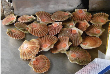
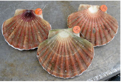
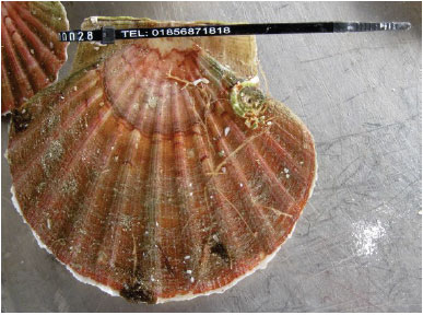
Legal scallops (≥100 mm shell width) were (mostly) retained for landing and a sample of (mostly) sub-legal scallops was tagged. Subsequent recaptures of scallops that had grown to legal size were returned to the survey ground rather than being retained for landing. Three different tagging methods were trialled (Figure 2): numbered disk tag wired to one ear of the scallop; numbered disk tag glued to the flat valve near the umbo; numbered cable tie inserted through a hole drilled through one ear of the flat valve. In addition to tagging, some scallops were marked with black mastic, enabling untagged resident scallops to be recognised on subsequent occasions.

Figure 2: Tagged scallops of three different types used in Orkney during 2013-2014.

(a) Glued disk tags

(b) Wired disk tags

(c) Cable tie tag

The depletion fishing experiments provide spot estimates of the scallop population (both tagged and untagged) present in the survey area on each occasion, whilst recaptures of tagged scallops provide a perspective on population dynamics between occasions. Application of the Cormack-Jolly-Seber ( CJS) model (Lebreton et al., 1992) allows recaptures to be modelled as a function of survival/fidelity and recapture probabilities. Recapture data are pooled between dives within survey occasions, thus recapture probabilities estimated from tagging are equivalent to the depletion estimates cumulated over the dives (Equation 2) ^[1] . The CJS model was implemented in Excel for this project, based on determining cell probabilities in 'reduced m-arrays' (Burnham et al., 1987). The reduced m-array format is a summary of the recapture data where rows of the array refer to release cohorts and columns refer to occasions of first recapture. Re-releases of tag recaptures are treated alongside new releases in following release cohorts (this is the 'reduced' element of the m-array). Data on release numbers, first recaptures and numbers never recaptured from each release cohort are sufficient for maximum likelihood estimation of all the parameters of a CJS model (Burnham & Anderson, 1987). Allowance was made for unequal sampling intervals (42-207 days) between occasions, so that meaningful equality constraints could be made for survival/fidelity probabilities, i.e. on a per day rather than per interval basis. Similar to the depletion model, 16 different CJS-type models were considered, based time * size, time, size and constant constraints on either or both of the survival/fidelity and capture probabilities. Logistic transformation was used to constrain all probabilities within feasible bounds. Model fitting was by maximum likelihood, with the kernel of a multinomial log-likelihood ( l) defined as:

, Eq. 3

where m _ij is an observed element of the reduced m-array, p _ij is the probability of that observation, formed in terms of survival/fidelity and capture probabilities and the summation is over the rows ( i) and columns ( j) of the reduced m-array. This log-likelihood was maximised using the Solver add-in in Excel.

A goodness-of-fit test for the full model ( time * size for both survival/fidelity and capture probabilities) was based on a Pearson _X ² statistic for the reduced m-array, with pooling of expectations <2 within rows. A non-significant value for this statistic (see below) indicates that the CJS model is a suitable basis for inference about recapture probabilities and that the tagging data were not over-dispersed with respect to the assumptions of a multinomial likelihood. Selection of the simplest adequate model as a basis for further inference was based on minimum value of the Akaike Information Criterion adjusted for small sample size ( AIC _c). Given several models with AIC _c values differing from the minimum by about two or less, final survival/fidelity and capture probability estimates were obtained by model averaging following the approach of Burnham & Anderson (2002). Survival/fidelity and capture probabilities from all models were estimated for each size-group and occasion, and weighted averages across the models were calculated using relative model likelihoods as weights ('Akaike weights'). The final probability estimates are thus most strongly influenced by the most likely model (model with lowest value of AIC _c), with other models contributing according to their relative likelihoods.

Given the use of Excel to fit the CJS-type models to the data, a variance-covariance matrix is not available for the model estimates, so a full exploration of uncertainty around model parameters is not yet possible. An implementation of the model in the R statistical package will allow this to be explored in future.

Permanent emigration cannot be distinguished from mortality in these CJS-type models, hence the reference to survival/fidelity probabilities. Given an assumed value for the instantaneous rate of natural mortality ( M) of 0.15 yr ^-1 for Scottish scallop populations (e.g. Dobby et al., 2012), it is possible to partition the two components. Given a survival/fidelity of ø, expressed on a daily basis, an assumed daily probability of fidelity f to the survey area can be calculated as:

, Eq. 4

This then allows the probability of permanent emigration E to be estimated for any given time interval to be calculated as:

, Eq. 5

where t is the interval duration in days.

Small Scale Movement Patterns

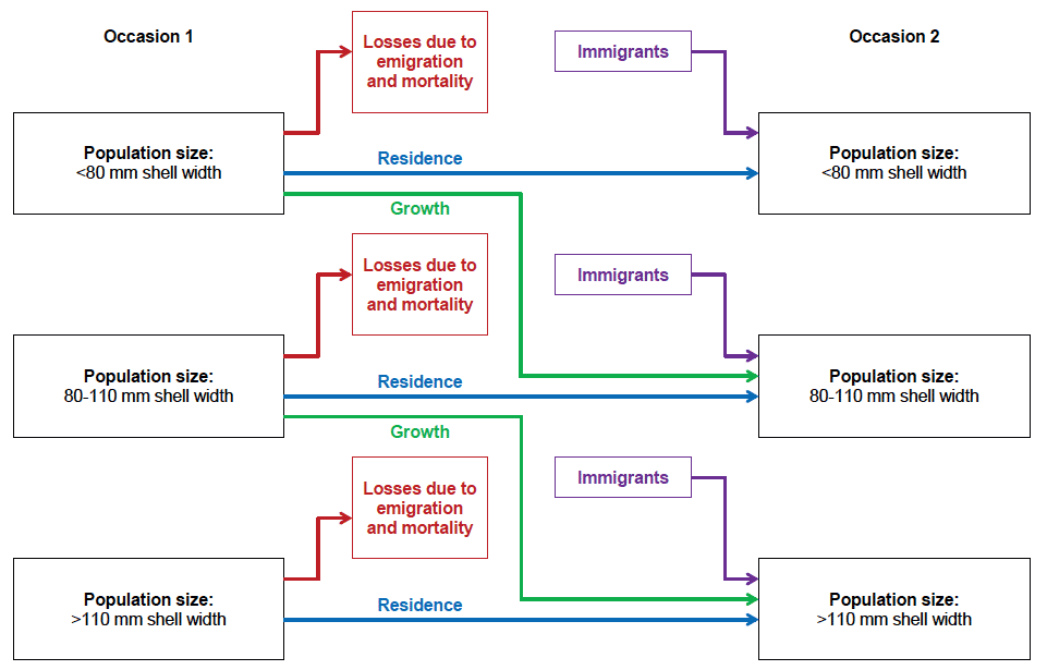
Estimates from the depletion and tagging experiments can be used to provide a complete picture of scallop population dynamics in the survey plot. As summarised in Figure 3, these processes are:

(i) Losses due to emigration and mortality. Removals of legal-sized scallops (≥100 mm shell width) by fishing are known. For size-group j, losses of scallops from the survey area due to permanent emigration or natural mortality between occasions i and i+1, L _ij, are given by:

, Eq. 6

where N _ij is the population number in size-group j estimated by depletion model for occasion i, F _ij is the number of scallops of that size-group removed by fishing, ø _ij is the daily survival/fidelity probability of scallops in that size-group during the interval between occasions i and i+1, and t _i is the duration of that interval in days.

(ii) Transition between size-groups owing to growth. The sizes of tagged scallops measured on consecutive occasions can be used to estimate the probabilities of transitions between size-groups. Growth between occasions can be represented by a linear relationship:

, Eq. 7a

where W _i and W _{i +1} are shell widths on occasions i and i+1 respectively, and a and b are the intercept and slope of the relationship, estimated by linear regression. The threshold shell width above which scallops grow into the next size-group is then estimated by inverting this relationship:

, Eq. 7b

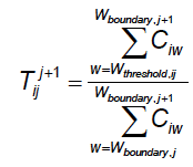
where W _{threshold , ij} is the threshold for shell widths in size-group j measured on occasion i, and W _{boundary , j +1} is the lower length boundary of the recipient size-group j+1. The probability of transition between size-groups j and j+1 between occasions i and i+1, T _{ij ,} is then:

, Eq. 8

where C _iw is the number of scallops of size w caught on occasion i (note that w indexes the multiple sizes that are grouped within a size-group). Note that transition probabilities estimated in this way are conditioned on the scallop size composition measured in the survey catches. This is appropriate for the accounting of population processes between surveys, but does not generalise to populations differing in size structure. Too few data are available to allow construction of a generalised transition matrix between size-classes defined at a finer level. Using the transition probabilities defined in Eq. 8, the number of scallops growing between size-group is calculated as:

, Eq. 9

where G _ij is the number in size-group j on occasion i that remains in the survey area on occasion i+1, having grown to size-group j+1.

(iii) Residency within the survey area and size-group. The number of scallops of size-group j that remain in the survey area between occasions i and i+1, without growing into the next size-group during that interval, R _ij is given by:

, Eq. 10

where all quantities are subscripted by occasion i and size-group j. This represents the starting population number from which fishery removals, emigration and growth of the remainder are subtracted.

(iv) Immigration into the survey area from outside. Once the processes of losses due to emigration/mortality, growth between size-groups and residency within the survey area have been projected between survey occasions, any discrepancy between the projected population and that estimated by the depletion model should in principle be accounted for by immigration of new scallops from outside the survey area:

, Eq. 11

where I _{i +1, j} is the number of immigrants into the population in size-group j measured at occasion i+1.

Figure 3: Diagram of population dynamic processes affecting changes in numbers of scallops in each size-group within the survey area between survey occasions.
Note that emigration accounted for among the losses is permanent within the time-scale of the survey series. Mortality of scallops larger than 100 mm shell width includes known fishery removals.