Marine piling - energy conversion factors in underwater radiated sound: review
A report which investigates the Energy Conversion Factor (ECF) method and provides recommendations regarding the modelling approaches for impact piling as used in environmental impact assessments (EIA) in Scottish Waters.
3. Sound Propagation from Point and Line Sources
As noted in the derivation of the source energy formula, there is a difference between the nature of sound propagation from a point and from a line. This section investigates the differences between the two firstly using geometrical models to provide a general overview of the differences, and secondly using numerical modelling of a basic benchmark scenario.
3.1. Geometrical Sound Propagation Models
The propagation of sound depends on many factors that typically require detailed modelling to assess accurately. However, in many cases geometrical models provide very useful insight into the nature of sound propagation, and providing they are used appropriately, can provide accurate results of losses with increasing distance from the source.
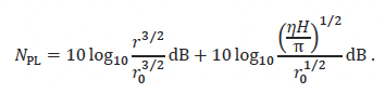
In deep water, for example, basing sound propagation loss, NPL, on spherical spreading, i.e.,
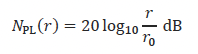
is a reasonable approximation up to distance where reflections from the seafloor become important.
In shallow water, which is more typical for piling, there exist simple expressions for propagation and transmission losses that take the shallow wave guide into consideration.
It is useful to distinguish between propagation loss and transmission loss. Both terms are defined in ISO 18405:
propagation loss: the “difference between source level in a specified direction and mean-square sound pressure level at a specified position”, and;
transmission loss: the “reduction in a specified level between two specified points x1, x2 that are within an underwater acoustic field”.
As described, the impacted pile does not have a source level, and consequently it is meaningless to use propagation loss in the calculation of received levels. Therefore, one needs to use transmission loss to characterise the change in level of the sound field with distance in the presence of the impacted pile.
3.1.1. Geometrical shallow water point source models
This section draws from work by Ainslie et al. (2014) from the conference paper “Practical Spreading Laws: The Snakes and Ladders of Shallow Water Acoustics” and presents the formulae for shallow water propagation loss when considering both monopole and dipole sources.
If one considers a point source, positioned in the water column suitably far from any boundaries, the initial sound propagation is in spherical shells located at the source. Consequently, sound propagation close to the point source is characterised by spherical spreading. In equation terms, the propagation loss, NPL, is
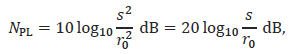
where s is the distance between the acoustic centre of the source and the receiver.
At greater distances from the source, the sea floor and sea surface have increasing influence over the sound field. The area through which the sound propagates becomes 2πrH where r is the horizontal distance from the source and H is the water depth. However, only sound propagating at angles less than the critical angle, Ψ, contributes to this cylindrical spreading region. This yields a vertical aperture angle of 2Ψ and a propagation loss of
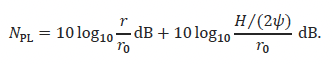
Here, the 10log10(r) term dictates this to be cylindrical spreading.
With additional bottom reflections, energy propagating at steeper angles become more rapidly dissipated than those travelling close to horizontal. Consequently, the effective aperture angle decreases with range and can be expressed as
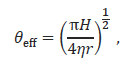
where η is the gradient of seabed reflection loss with angle in units of nepers per radian (Np/rad).
Replacing 2Ψ with the effective range-dependent aperture angle provides a propagation loss of
Here, the 10log10(r3/2)=15log10(r) corresponds to the standard mode-stripping formula.
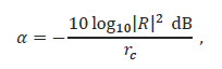
These three propagation loss equations illustrate the three different regions of spreading involved in sound propagation from a point source comprising spherical spreading, cylindrical spreading, and mode-stripping (or intermediate) spreading. Whilst there are simplifications and assumptions involved, they are accurate enough for many applications, particularly in favourable environments or for continuous sources operating over a narrow band of frequencies suitably far from the boundaries.
For point sources close to the boundary, Ainslie et al provide similar equations representing the point as a dipole source. Here, the point source sound field is strongly influenced by the reflected sound field, with the reflection providing a phase shift of 180° which gives rise to a Lloyd mirror interference pattern.
Figure 7 shows the propagation loss for a monopole point source calculated using the equations above.
3.1.2. Damped cylindrical spreading
The impacted pile, as an acoustic source, behaves rather differently from a point source. The sound generation starts with the hammer impact at the top of the pile. This creates a compressive wave that travels down the pile at the compressive wave speed of steel. Associated with this wave is a localised radial expansion at the pile wall resulting in an acoustic wave travelling from the pile wall outwards. Taking the entire wetted pile length as the radiating surface results in conical wavefronts, or ‘Mach’ waves, the angle of which is dictated by the relative speeds of the compressional wave in water and steel.
The wavefronts radiate from the pile travelling at the angle of the cone. The sound then bounces between the seafloor and the sea surface losing energy with each reflection. As the energy of interest exists across the entire water column and is contained within it, the propagation resembles that of cylindrical spreading. The repeated bounces, however, provide an attenuation in level that is proportional to the distance from the pile.
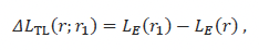
The DCS model (Lippert et al. 2018) characterises the sound propagation based on the physical description. One important aspect to note, however, is that because source levels do not exist for piling, use of the term propagation loss in this context is meaningless. It therefore makes more sense to use transmission loss, described above as the change in sound level between two points in an acoustic field.
The transmission loss between points at ranges r and r1 from a source is given by
where LE is the sound exposure level. For sound radiated by the pile, the sound energy is spread into an area of 2πrH, where H is the water depth; this corresponds to cylindrical spreading. In addition to this, there is the energy loss from multiple boundary reflections causing exponential decay. With these two elements, the DCS model can be written as
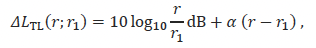
where the horizontal decay rate, a, is given by
is the plane wave reflection coefficient, and rc is the horizontal distance between successive bottom reflections.
The DCS model has been validated against measurements that has found good agreement up to a limiting range dictated by the attenuation coefficient (Ainslie et al. 2020). The maximum usable range of Equation 23 is dictated by the a term. Where ar becomes large the amplitude of the Mach cone becomes negligible compared to the near-horizontal paths that are initially much weaker. An upper limit of ar < 20 dB has been suggested based on measurements, after which an extrapolation scheme using 25log10(r) is applied (Heaney et al. 2020).
An example of transmission loss calculated using the DCS model is shown in Figure 8.
3.1.3. Comparison of point monopole source propagation and DCS
Given the differences in the nature of propagation between the point source and the DCS model it is informative to provide a direct comparison. Here, we consider three basic examples illustrating how the curves can diverge.
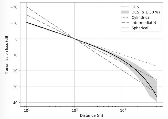
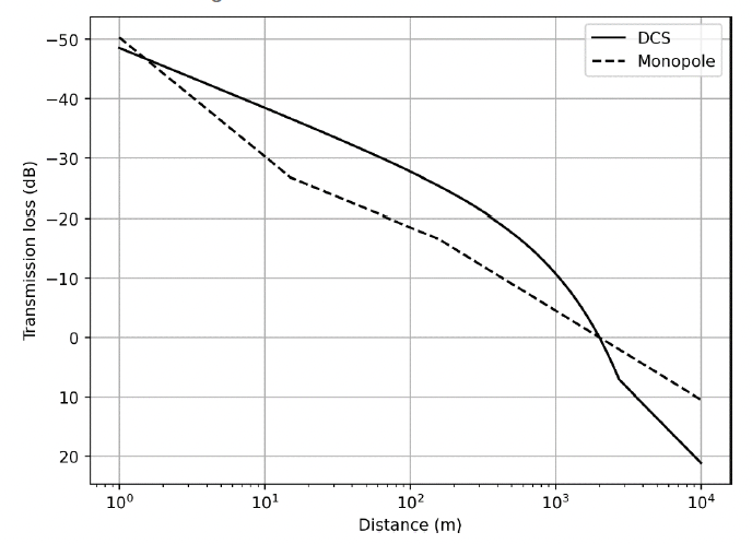
In the first example, we consider a situation featuring a sound source in a water depth of 30 m. Figure 9 shows the transmission loss curves calculated using the monopole model, and the DCS model presuming a reference distance of 100 m from the source in a best-case scenario. In this instance, the propagation from the monopole source is in the cylindrical spreading region, and consequently the curves match reasonably well from 30 to 1000 m. The differences near the source are due to the spherical spreading regime of the monopole, and differences at greater distances are caused by the increasing significance of the absorption term in the DCS model. Level differences at 1, 100, and 5000 m are shown in Table 3.
| Distance from source (m) | Monopole ΔLTL | DCS ΔLTL | Difference in ΔLTL |
|---|---|---|---|
| 1 | -34.8 | -20.4 | 14.4 |
| 100 (reference) | 0 | 0 | 0 |
| 5000 | 23.0 | 36.0 | 13.0 |
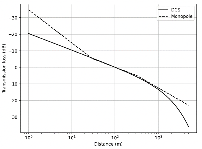
The second example considers the effect of increasing the water depth to 100 m, with all other parameters kept constant. The reference point again is 100 m. Figure 10 shows the transmission loss relative to the sound level at 100 m for this deeper case. Here, the deeper water results in the point source propagation to exist in the spherical spreading regime for longer, such that sound levels close to the source diverge more between the two models than for the previous example. The cylindrical spreading region for the point source model starts at 100 m. Due to the deeper water, the propagating wave from the pile experiences fewer reflections for a given distance such that the absorption term is reduced; this results in the two curves agreeing over a longer distance. Inevitably, however, at increasing distances the absorption term in the DCS model dominates such that at greater ranges the point source model still overpredicts the sound levels. Calculated transmission losses for select points are shown in Table 4.
| Distance from source (m) | Monopole ΔLTL | DCS ΔLTL | Difference in ΔLTL |
|---|---|---|---|
| 1 | -40.0 | -20.1 | 19.9 |
| 100 (reference) | 0 | 0 | 0 |
| 5000 | 20.4 | 22.7 | 13.0 |
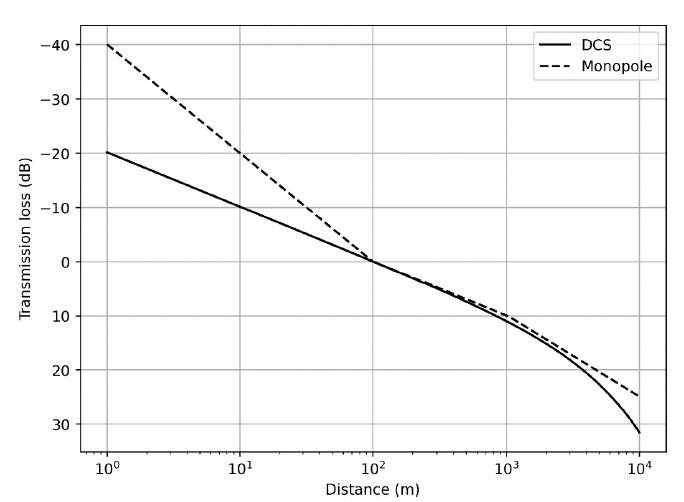
The third and last example to be considered here illustrates how different circumstances, taking different reference points and different environments, can lead to different outcomes. Using a reference distance of 2 km, and a water depth of 15 m, whilst keeping everything else constant results in the curve seen in Figure 11. Here, there are substantial differences between the nature of sound propagation between the two models leading to significant errors if one were to use the incorrect method as shown in Table 5.
| Distance from source (m) | Monopole ΔLTL | DCS ΔLTL | Difference in ΔLTL |
|---|---|---|---|
| 1 | -50.3 | -48.5 | 1.8 |
| 100 | -18.5 | -27.7 | -9.2 |
| 5000 | 6.0 | 13.7 | 7.7 |
We present a worked example of sound level predictions when using two of these transmission loss curves. In the first example, with 30 m water depth and a reference distance of 100 m, if the measured SEL was 190 dB, the predicted theoretical levels at 1 m would be 224.8 dB for the monopole source compared to 210.4 dB from the DCS model. Similarly, at 5 km, the monopole model would generate an SEL of 167.0 dB compared to 154.0 dB from the DCS models.
Often the primary output from the modelling comprises predictions of distances at which sound levels drop below specified threshold levels as shown in Table 6. It is noted that the results presented here all consider just the broadband sound level, i.e., no frequency-weighting has been applied. Using the first example from Figure 9, comparing distances to where the SEL drops to 180 dB, the monopole provides 690 m compared to 640 m from the DCS model. However, a similar comparison where the SEL drops below 170 dB yields 3.1 km for the monopole compared to 2.0 km from the DCS model. The differences in this case, increase as one moves further from the reference distance.
In the shallow water case in the third example shown in Figure 11, if one were to presume a measured SEL of 170 dB at 2 km, the result at 1 m is 220.3 dB for the monopole and 218.5 dB for the DCS model. Whilst the similarity in levels at this distance looks encouraging, the intervening SEL results depart substantially from one another. At 100 m, we see a predicted SEL from the monopole model of 188.5 dB but 197.7 for the DCS model. Again, looking at distances to where the SEL drops below a certain value (Table 7), for 190 dB the distances are 73 m for the monopole model and 370 m for the DCS model; for 180 dB, these are 430 m and 1.1 km respectively.
| SEL threshold (dB) | Monopole model distance (m) | DCS model distance (m) |
|---|---|---|
| 190 (reference) | 100 | 100 |
| 180 | 693 | 640 |
| 170 | 3183 | 1950 |
| SEL threshold (dB) | Monopole model distance (m) | DCS model distance (m) |
|---|---|---|
| 190 | 73 | 374 |
| 180 | 434 | 1084 |
| 170 (reference) | 2000 | 2000 |
The examples above illustrate the need to use an appropriate model for each situation. We have not presented any results using the dipole source geometric model; however, given the varied spreading regimes, it is clear that the end result would show that this is also very different from the DCS model. It is noted that while the geometric model differs from the DCS model, more sophisticated point source modelling will generate more accurate answers for situations involving more complex environments and signals. To further illustrate that, despite this, the point source model is inadequate for piling predictions, we provide examples using numerical modelling in the next section.
3.2. Numerical Sound Propagation Modelling
While geometric models provide very quick answers and useful insight to the problem, it can be argued that they are not suited to all situations and that more sophisticated methods are required. This section provides two simple examples of numerical modelling results when considering propagation from both a point source and a line source.
3.2.1. Example scenario
The parameters used for the baseline scenario are selected to be broadly typical of a North Sea piling operation. The pile properties are shown in Table 8. The hammer selected for the study was an IHC S‑2300 operating at its full capacity of 2300 kJ. The choice of hammer is based on using one that has been commonly used for monopile installation and is not intended to imply a recommendation.
Table 8. Parameters for the example pile.
Pile length: 70.0 m
Pile diameter: 6.0 m
Pile wall thickness: 5 cm
Penetration depth: 20.0 m
The environment comprised a 30 m column of water and flat bathymetry. The sound speed profile for the study is an isovelocity profile at 1490 m/s. The sediment is based on medium sand, with a grain size of 1.5 φ. The geoacoustic profile in Table 9 has been calculated using surficial sediment properties taken from Ainslie (2010) and depth-dependent equations from Hamilton (1980); shear wave properties are from general results by Holzer et al. (2005) and Buckingham (2005).
| Depth below seafloor (m) | Material | Density (g/cm3) | Compressional wave | Shear wave | ||
|---|---|---|---|---|---|---|
| Speed (m/s) | Attenuation (dB/λ) | Speed (m/s) | Attenuation (dB/λ) | |||
| 0 | Sand | 2.090 | 1784.7 | 0.88 | 300 | 3.65 |
| 100 | 2.216 | 1908.0 | 0.85 | |||
| 200 | 2.337 | 2017.9 | 0.81 | |||
| 300 | 2.447 | 2116.2 | 0.76 | |||
| 400 | 2.546 | 2204.2 | 0.71 | |||
| 500 | 2.634 | 2283.6 | 0.66 | |||
3.2.1.1. Line source modelling
To perform the numerical modelling for the phased line source JASCO’s PDSM (MacGillivray 2014) was used. The process involves the following steps:
- Define the input forcing function at the head of the pile using GRLWEAP (Pile Dynamics 2010).
- Model the progression of the stress wave down the pile based on a finite-difference calculation of cylindrical shell equations, whilst taking the radiation damping of the water and sediment, and the pile toe reflection into account.
- Calculate the contributions of an array of monopoles located on the central axis that simulate the radiated sound field at the pile wall.
- An array starter method is used to generate a directional starting field at each frequency to fully take into account the geometry of the source.
- The starting field is propagated in distance using a parabolic equation model (described above).
Further details of the model used for the line source in this example are provided in Appendix A. The monopoles on the central axis were positioned 1 m apart, and the maximum frequency of the model was 1123 Hz (upper band edge of the 1 kHz decidecade band). The parabolic equation model used a frequency-dependent range step between 50 m at the lowest frequencies to 10 m at the highest; similarly, the depth step ranged from 0.5 m to 0.125 m.
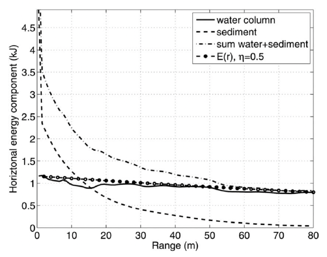
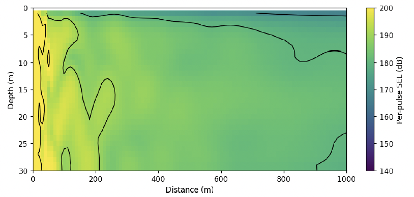
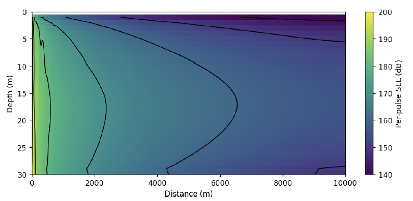
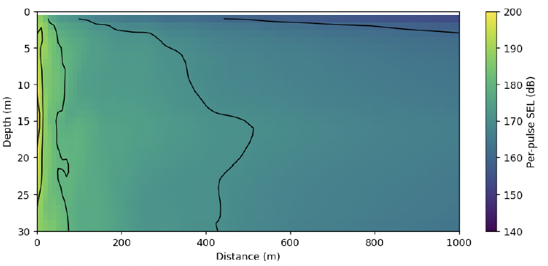
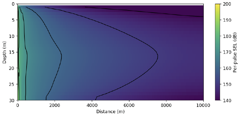
Figures 12 and 13 show the per-pulse SEL field calculated by the line-source model over 1 km and 10 km respectively. In Figure 12, the path of the Mach wave, and associated shadow zone are visible at ranges up to approximately 150 m.
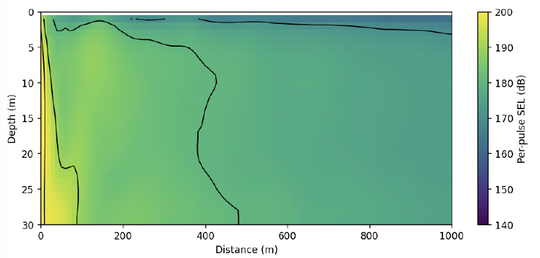
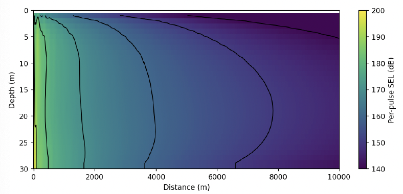
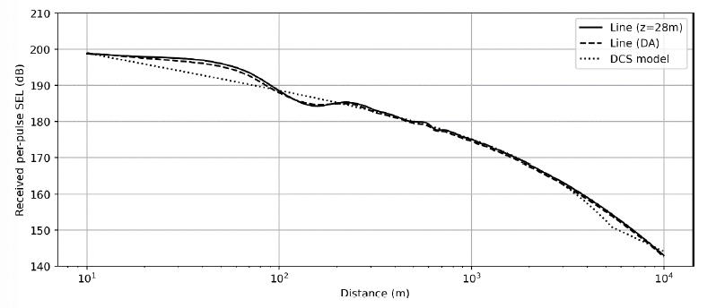
Figure 14 shows the per-pulse SEL both for a receiver 2 m from the sea floor, the depth-averaged result, and the DCS model. As the DCS model only provides predictions of transmission loss, it is necessary to include a measured or modelled received level to generate full level against range results. In this case, sound levels were matched at 10 m from the pile, but it is evident that there would be small errors if the sound levels were matched at a point where the curves separate (i.e., 50 m or 150 m). Additionally, as stated in Section 3.1.2, the DCS model is less suited to greater ranges where the absorption term is great and other mechanisms giving rise to sound energy travelling near horizontally start to dominate; this is evident in the plot from approximately 4 km, with the empirical change to 25log10(r) propagation starting from 5 km.
3.2.1.2. Point source modelling using sample measurements
Where measurements are available, a commonly used method for calculating the sound field is to take the result at the measurement point, back-propagate it to a source location, and forward-propagate in order to generate the full sound field. Results from Figure 14 suggest that when using an appropriate model, this approach may yield very reasonable outcomes. In this case, however, we investigate the effect of basing propagation loss on a point source assumption.
Point source propagation losses were calculated in RAM (see Section 2.2.2) for a source located at 15 m depth (i.e., mid-depth) for decidecade band centre frequencies from 10 Hz to 1 kHz for the environment described above. Results for the decidecade bands were generated from the single frequency propagation loss using a frequency averaging algorithm (Harrison and Harrison 1995).
Results are calculated for receivers located at 100 m and 170 m from the pile, both 2 m from the seafloor. Back-propagating for each decidecade band provides two very different source level spectra as shown in Figure 15. Whereas the structure of the sound field for the pile varies little with frequency (as energy is travelling in the fixed direction), the sound fields resulting from the point sources have more structure that varies with frequency. Consequently, in cases where incorrect propagation losses are used, it is possible to generate large differences between back-propagated source levels simply due to location of the measurement point. Here, we see source levels taken from 100 m receiver to be significantly higher than those for the 170 m receiver; additionally, the peak frequency has moved from the 160 Hz band to 63 Hz. The broadband source levels of the two results are shown in Table 10.
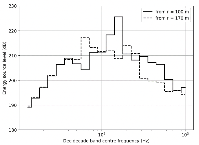
Table 10. Broadband energy source levels (dB re 1 µPa²m²s) calculated using the back-propagating from a single point.
Parameter - ESL (dB)
From 100 m - 227.2
From 170 m - 222.4
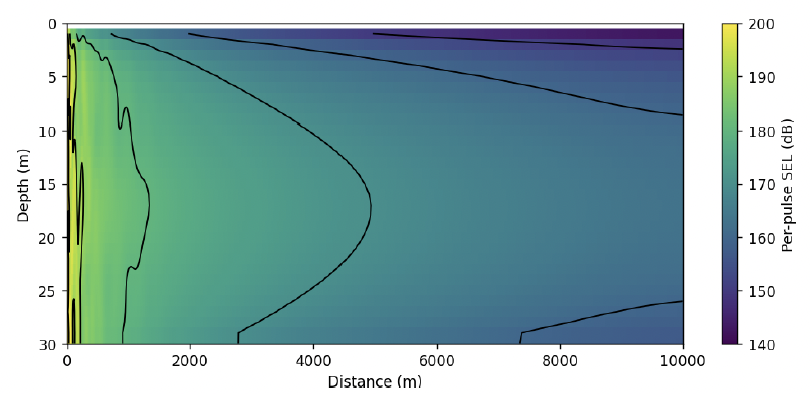
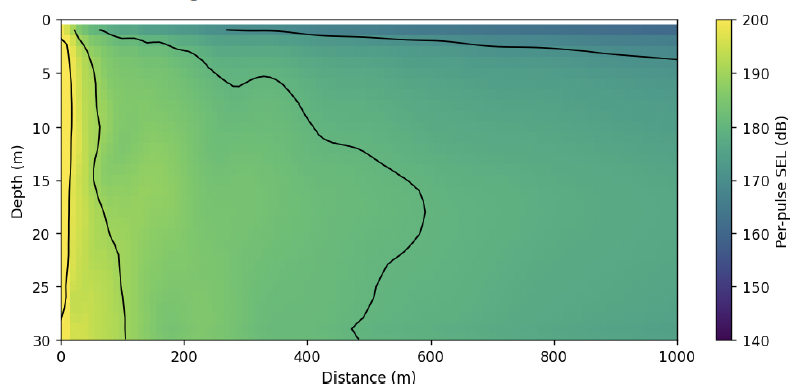
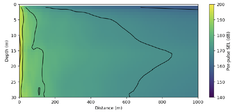
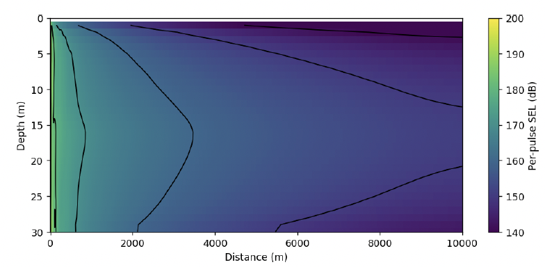
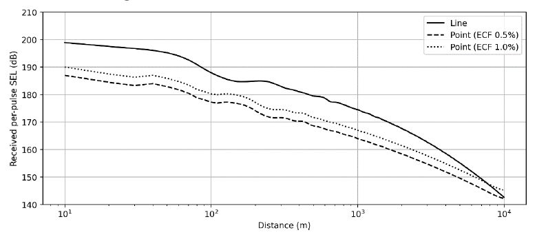
Figures 16 and 17 show the calculated sound field up to 1 km and 10 km respectively for source levels calculated at 100 m. Similarly, Figures 18 and 19 show the calculated sound field up to 1 km and 10 km respectively for source levels calculated at 170 m.
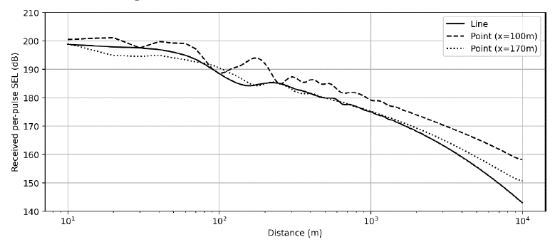
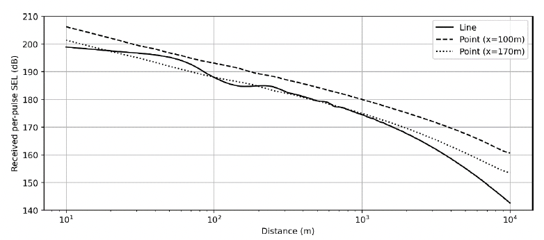
Figure 20 shows the calculated per-pulse SEL taken at a depth of 28 m as a function of distance from the pile for the line-source and the two point-source outputs. Here, we note that the levels for the point source are matched to the line source at their respective distances. Figure 21 shows the equivalent depth-averaged results. Here we see a poor match for source levels calculated at 100 m, but a reasonable match for the first couple of kilometres for the source levels calculated at 170 m. For much of the range, the point source field is in the cylindrical spreading region, which is similar to the DCS model where the absorption term is still low. Once out of this region, however, the exponential losses apparent in the DCS model cause the curves to diverge. It’s also worth noting that although in this case there was a reasonable match between the line source and the point source from 170 m levels, as shown, the back-propagated source levels can vary substantially based on the location from which they are calculated.
3.2.1.3. Modelling using point-source equivalent ECF method
The final example presented in this section is for modelling using the point-source equivalent ECF method. Here the broadband energy source level is calculated using Equation 1, for the given hammer impact energy of 2300 kJ. The calculated energy source levels are shown in Table 11 for point-source equivalent ECFs of 0.5 % and 1.0 %.
Table 11. Broadband energy source levels (dB re 1 µPa²m²s) calculated using the point-source equivalent ECF method.
Parameter: ESL (dB)
ECF: 0.5 % - 211.5
ECF: 1.0 % - 214.5
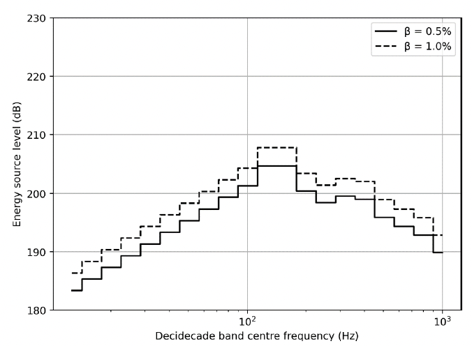
The spectral shape of the source is taken from a figure of the source spectrum presented in Moray East underwater noise modelling report (Cefas 2019). The relative contribution between the frequency bands is constant, with levels offset to provide the broadband levels from Table 11. The resulting ESL spectra are shown in Figure 22.
Comparing the energy source levels between those generated using the point-source equivalent ECF method (Table 11) and those using the back propagated value (Table 10) shows that, in this particular case, the point-source equivalent ECF method generates substantially lower source levels.
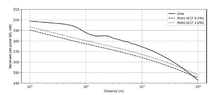
The propagation loss calculations from the point source model in Section 3.2.1.2 were reused for the point-source equivalent ECF-derived source levels. Slice plots of the sound fields up to 1 km and 10 km from the pile for the β = 0.5 % ECF source are shown in Figures 23 and 24, with equivalent results for β = 1.0 % in Figures 25 and 26. Comparing against the equivalent results for the back-propagated sound levels, the point-source equivalent ECF method in this example produces substantially lower sound levels in the field.
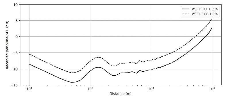
Depth-averaged values for the two point-source equivalent ECF method results were calculated to compare against the line source model result and are shown in Figure 28. Here, we see large differences between the ECF results and the line source not only in terms of the sound level difference but also in the rate of decay as a function of range as shown in Figure 29.
3.2.1.4. Comparison of results
The methods presented in this section comprise a line-source model designed specifically to predict sound levels from piling, a point source model where there is a reference measurement at some point, and the same point source model using the point-source equivalent ECF method to generate source levels. In the case of using the DCS model, sound levels need to be obtained either from measurements or from a very similar previous study. The match against the line-source model, however, is good when taking a suitable reference point (Figure 14).
The point source examples using the refence sound level again illustrate the differences in the sound field between the different source assumptions. It also illustrates the possible differences that result from having a different reference location. In this case, the reference point of 170 m results in a reasonable match between the line and point source for the distances shown in the plot. This, however, should not lead one into thinking that this a suitable method, as taking a reference level at 100 m results in completely different propagation due to the implied prominence from different frequencies (see Figure 15). It is also evident that one cannot determine a good matching reference without having initially performed the appropriate modelling.
The point-source equivalent ECF method offers an alternate method of determining source levels directly without needing to back-propagate existing sound levels. Here, as previously described, spectral levels from measurements are increased or decreased in level to match a broadband ESL that is calculated from the hammer energy and the point-source equivalent ECF (Figure 22). In the example presented here, the broadband source levels for the point-source equivalent ECF method (211.5 and 214.5 dB) was substantially lower than either of those from the back-propagated results (227.2 and 224.0 dB). The result of this is that ECF model sound levels in this example differ by 7 to 12 dB between 100 and 1000 m from the pile (Figure 29), and feature very different loss beyond 2 km.
As stated previously, a sought-after output of the modelling is often the distance at which sound levels drop below given thresholds. Table 12 provides an indication of the spread of values from the models in this example. It also highlights the importance of the source function used in the modelling; here we see the results from the ECF model falling far short of those from the other results when using the most commonly used values of the ECF.
| Depth-averaged per-pulse SEL (dB) | PDSM | Point source | |||
|---|---|---|---|---|---|
| Back-propagated ESL | point-source equivalent ECF ESL | ||||
| r = 100 m | r = 170 m | β = 0.5 | β = 1.0 | ||
| 190 | 0.09 | 0.18 | 0.07 | 0.02 | 0.02 |
| 185 | 0.14 | 0.45 | 0.20 | 0.03 | 0.05 |
| 180 | 0.46 | 1.00 | 0.45 | 0.07 | 0.11 |
| 175 | 0.93 | 2.03 | 0.99 | 0.16 | 0.28 |
| 170 | 1.61 | 3.81 | 1.89 | 0.39 | 0.65 |
| 165 | 2.50 | 6.46 | 3.27 | 0.89 | 1.38 |
| 160 | 3.63 | >10.0 | 5.30 | 1.81 | 2.66 |
3.2.2. COMPILE II benchmark scenario
We briefly consider here a second modelled scenario based on the COMPILE II workshop scenario. The COMPILE II case was a real-life pile driving scenario with no noise mitigation measures, for which measurement data was made available after results submission for validating the acoustic models. Here, we present results generated by PDSM and those for the point-source equivalent ECF model with values for β of 0.5 % and 1.0 % for the COMPILE II benchmark scenario.
3.2.2.1. Scenario description
The scenario describes a 75 m long pile, including a taper to bring the pile diameter from 5 m to 6.5 m over 20 m in the mid-section, being driven by a Menck MHU-3500S hammer. At the point of measurement, the blow energy was 1525 kJ and the pile had been driven 30 m. The water depth varies in accordance with Table 13 with participants instructed to obtain intermediate water depths through linear interpolation and assume constant bathymetry beyond the maximum distance. The pile was driven into layered sand and clay.
| Distance (m) | Water depth (m) |
|---|---|
| 0 | 39 |
| 245 | 39 |
| 747 | 37 |
| 1481 | 32 |
The sound speed profile for the study is an isovelocity profile at 1500 m/s. The geoacoustic profile (Table 14) was calculated from geological data provided for the workshop based on Buckingham’s grain-shearing model (2005).
| Depth below seafloor (m) | Material | Density (g/cm3) | Compressional wave | Shear wave | ||
|---|---|---|---|---|---|---|
| Speed (m/s) | Attenuation (dB/λ) | Speed (m/s) | Attenuation (dB/λ) | |||
| 0–5.0 | Loose to medium dense sand | 2.05-2.05 | 1696.0-1892.7 | 0.26-0.93 | 106.3-389.4 | 3.65 |
| 5.0–6.5 | Dense to very dense sand | 2.09-2.09 | 1912.9-1940.3 | 0.9-0.98 | 391.3-426.1 | |
| 6.5–9.0 | Sandy clay | 2.08-2.08 | 1707.3-1713.7 | 0.23-0.26 | 95.7-106.3 | |
| 9.0–11.5 | Dense to very dense sand | 2.09-2.09 | 1976.6-2008.9 | 1.08-1.16 | 475.4-515 | |
| 11.5–19.0 | Sandy clay | 2.08-2.08 | 1719.4-1732.3 | 0.28-0.33 | 115.9-136.2 | |
| 19.0–50.0 | Very dense silty sand | 2.09-2.09 | 1908.1-2022.6 | 0.89-1.19 | 383.6-531.4 | |
3.2.2.2. Modelling assumptions
The point source model has been calculated for point-source equivalent ECFs of 0.5 % and 1.0 % based on the source spectrum shown in Figure 22, and the input hammer energy of 1525 kJ. The point source depth has been chosen as half of the water depth. Identical environments have been used for both the point source and line source modelling.
3.2.2.3. Results
Figure 30 shows the modelled per-pulse SEL 2 m from the seafloor against distance from the centre of the pile for the PDSM and point source results, along with the measurements made. Figure 31 shows the equivalent depth-averaged results against distance.
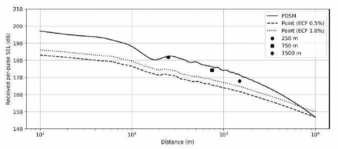
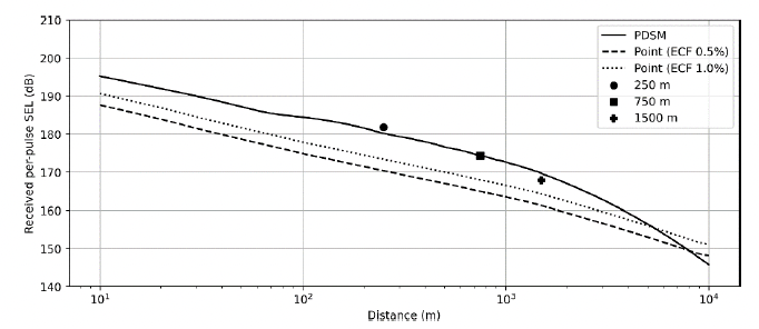
As seen in the previous study, the point-source equivalent ECF model is a poor predictor of sound levels from impact piling. In this case, the sound levels at the receiver locations were underestimated by between 3.3 dB (1500 m receiver, β = 1.0 %) and 10.2 dB (250 m receiver, β = 0.5 %).
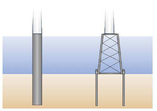
3.3. Consideration of Pin Piles
The examples shown in the previous sections principally consider the driving of monopiles. As more wind farms are built in deeper locations there is increased need for the installation of jacket structures. In construction, the jacket structure is deployed on the seabed and secured using a post-piling approach. This involves inserting piles into the skirt sleeves and driving the piles to secure the foundation. Figure 32 shows a drawing of the two foundations.
One key difference between the monopile and jacket pile installations is that in the case of the monopile the pile spans the entire water column at all points in the driving operation, whereas for the jacket pile the wetted length of the pile reduces over the piling sequence. In terms of radiated sound, the same acoustic mechanisms occur in that the stress wave travels down and up the pile producing wavefronts that propagate at the distinctive Mach angle. The reduction of the radiating area in water of the pin pile results in a reduction in radiated sound presuming all other parameters, such as the hammer energy, remain constant.
The point at which the radiated sound energy is a maximum, therefore, is determined by the combination of the hammer energy and the remaining stick-up length of the pile. The effect of the stick-up length on the radiated sound from the impacted submerged pile was studied by Lippert et al. (2017). It was found that, for the piles in question (2.44 m outer diameter, 82 m length, 40 m water depth), the change in SEL due to a change in wetted pile length could be calculated as 2.5 dB per 50% reduction in the remaining length of pile above the seabed. Consequently, when considering the worst-case assessment, it is most likely to occur at a point where there is a substantial portion of the pile still in the water column which may not correspond to the maximum hammer energy.
At points where there is little exposed pile in the water column, the propagation is unlikely to follow that of the DCS model. As stated, however, most interest will be at points where there is still much of the pile in the water column due to the associated higher sound levels. At these points, it is still necessary to consider the pile to be a line source generating wave fronts at the Mach angle rather than a point source.
3.4. Sound Propagation Summary
It has been shown in scientific literature that the nature of the propagation of sound from an impacted pile is substantially different from that for a point source. The sound field from the pile constitutes conical wavefronts known as the Mach cone, the angle of which is dictated by the relative sound speed of the water and down the pile. Point monopole sources, conversely, have multiple regimes of propagation initially comprising wavefronts in spherical shells, before transitioning to a cylindrical spreading regime some distance away, with a transition to a mode-stripping region beyond that.
This section provided an investigation into potential differences between generated sound fields based on the propagation assumptions. Examples were shown using geometric models, that take into account the general characteristics of the different propagation regimes, and numerical models, that fully account for the environment and the detailed propagation of the sound wave through the water and sediment.
In the case of the geometric models, results for a single point source were compared to the DCS model. It has been noted that the DCS model provides calculations of transmission loss rather than propagation loss; consequently, it requires a point of reference of another received sound level to generate the sound level as a function of range. Also, whilst the geometric monopole source results clearly show the transition between regions, the transitions are less clear for real environments and more complex source functions.
In the first two geometric examples shown (Figures 9 and 10), the sound levels between the two models were matched at 100 m for a favourable choice of parameters. As this corresponded to the cylindrical spreading regime in the monopole model, the two curves had a reasonable fit over much of the ranges of interest. Where deeper water was considered, there is a greater distance between successive bounces in the DCS model. Consequently, the absorption term takes longer before it starts to dominate, such that the propagation appears cylindrical over longer ranges. In the point source model, the water depth dictates the points at which the spreading regime changes; deeper waters result in an increased distance before propagation changes from spherical to cylindrical.
In the unfavourable case (Figure 11), absorption losses in the DCS model became substantial earlier due to the shallower water. Here, the transmission loss curves were matched at 2 km; however, the two types of propagation resulted in large level differences at ranges from 10 to 1000 m. In the cases of deriving sound levels, although the transmission loss curves can often be made to match for a certain distance, the rate of transmission loss diverges both close to the source and at greater distances where the absorption term in the DCS model starts to influence the result. At large enough distances, the point source model will always underpredict the transmission loss.
Two numerical examples were provided which are representative of typical modelling for impact assessments. In both cases, sound field levels generated by the point source models differed greatly from those of the line source model. The numerical model matched the general fit of the DCS model and provided a better match against measurements for a benchmarking study. Comparisons were shown against examples of the point-source equivalent ECF model. In these cases, using conversion factors of 0.5 % and 1.0 % underpredicted the sound levels within a few kilometres from the source. Although not shown, it’s clear that using a higher conversion factor (i.e., 4 %) would bring sound levels closer to the line source prediction nearer the source; at large distances, however, this would result in increasing overprediction of sound levels, and therefore an overestimate of distances to sound level isopleths.
Contact
Email: ScotMER@gov.scot