Improving understanding of seabird bycatch in Scottish longline fisheries and exploring potential solutions

Section 2: Statistical analysis of existing data

2.1 The data

Data used in this analysis were collected by onboard observers and were recorded on a haul-by-haul basis. The data covered a wide range of operational, environmental and catch data including, inter alia, the number of hooks set, line length, soak time, haul start/end times, date and position. The number of bycaught seabirds was recorded by species as the line was retrieved. Bycatch also occurred as the line was retrieved but these specimens were unhooked and are generally released alive. Live bycatch typically appears to form a small part of the total bycatch (circa 6%) but is highly variable and on some observed trips live bycatch exceeded the levels of dead bycatch. Only bycaught birds recorded as “dead” have been used in this analysis.

Most observed hauls (74%) had zero bird bycatch mortalities, and 92% of hauls had three or less bycatches. Counts of bycaught fulmars were highly over-dispersed with a variance to mean ratio of 6.99. Although fulmars accounted for most of the birds recorded, there were also ten northern gannet (Morus bassanus), two great shearwater (Ardenna gravis) and one great skua (Stercorarius skua) mortalities recorded.

The preliminary bycatch estimates for the longline fishery produced by Northridge .et al.(2020) were based on 14 trips sampled between 2010 and 2018. Sampling in the fishery continued after 2018, and by June 2021 observers under the BMP had undertaken a further four trips. Revised preliminary estimates were produced in summer 2021 incorporating all the data collected from 2010 to June 2021 using a similar analytical approach to Northridge et al.(2020). These updated estimates are presented in Section 3. A further five trips were also sampled between August and November 2021, increasing the total number of observed hauls from 103 in 2018 to 201 by the end of 2021, effectively doubling the amount of available data since the Northridge et al.(2020) report. The full 201 haul dataset was subsequently (late 2021) used to produce estimates for four species: northern fulmar, northern gannet, great skua and great shearwater using a modelling approach, rather than the ratio-based approach used in the earlier preliminary and revised preliminary estimates. Modelled estimates are provided in Section 3.

An important initial objective in our analysis was to examine how representative of the wider fleet activity the sampling data were. It is likely that the sample dataset contains significant biases, as hauls are not sampled in a truly random manner across the fleet, and haul observations are constrained by the fact that an observer must remain on the same vessel for the full duration of a trip.

The mean number of hauls per trip was 8.7 (95% confidence interval: 6.9 – 10.7). When hauls were considered within trip there was no evidence for any temporal clumping of the data (from a runs test on the per haul bycatch) for any of the bird species observed bycaught.

2.2 Are sampling data representative of fleet activity?

The UK offshore longline fleet undertakes approximately 500 trips per year. Annual sampling coverage in the longline fishery has been limited and largely carried out on a sporadic and opportunistic basis since 2010. By the end of 2021 a total of 23 trips and 201 hauls had been observed, meaning sampling coverage was typically less than 0.5% of total effort (in trips) per year. Total sampling effort in the fishery over the last decade equates to about 5% of the annual UK fishing effort in a typical year. According to official fishing effort statistics the UK longline fleet consisted of approximately 40 vessels since 2010 but this is misleading. Some vessels involved in the fishery have changed over the years and vessels may also change ownership and names, but usually there are about 10 to 15 vessels actively operating in any one year. Sampling trips have been undertaken on six different vessels between one and five times each. The selection of sampled vessels is essentially opportunistic and is based on the willingness of skippers and owners to carry observers. All sampled vessels so far are members of one of the two main industry representative organisations involved in the fishery.

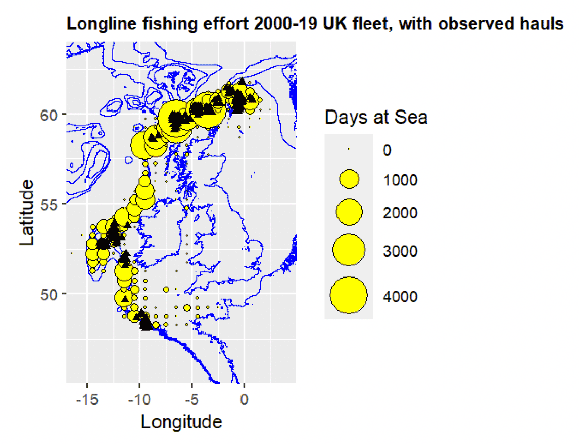
Making robust comparisons between low level sampling effort and overall fleet fishing effort for this fishery is not straightforward because the distribution of fishing effort is variable and relatively unpredictable within and between years. As an initial overall comparison Figure 1 shows the distribution of fishing effort by the UK offshore longline fleet (defined here as vessels over 20m in length targeting hake and to a much lesser extent ling (Molva molva) over the period 2000 to 2019 and sampling effort over the period 2010 to 2021. Yellow circles denote fishing effort by the fleet (in days at sea by ICES rectangle), while black triangles denote the sampled haul locations. Fleet effort has been mainly concentrated along the continental shelf edge especially North of Scotland. Sampled hauls are mainly north of Scotland, but also west and south of Ireland. Depth contours of the coastlines, 200m, 500m and 1000m isobaths are also show for context.

In general, there is reasonable agreement between the distribution of sampling and fleet fishing effort but given the low coverage levels it is expected that there would be some areas that are not particularly well represented. Sampling appears to have been relatively over-emphasised in the more northerly region and relatively under-emphasised between about 53^o N (Northwest Ireland) and 58^o N (West Scotland) and at around 51^o N (Southwest Ireland).

The relationship between fleet effort and observer sampling effort is demonstrated more clearly by examining the difference between the proportions of sampling to fishing effort along a latitudinal axis over the period 2010 to 2019. Figure 2 shows how the proportions of sampling, by half a degree of latitude (equivalent to the latitudinal dimension of an ICES rectangle) corresponds to the distribution of fishing effort. Values close to the 0% Y- axis indicate that the proportion of sampling is close to the proportion of fishing effort at that latitude. Values strongly negative indicate proportionally less sampling effort than fishing effort, while values with strongly positive values indicate proportionally more sampling effort than fishing effort.

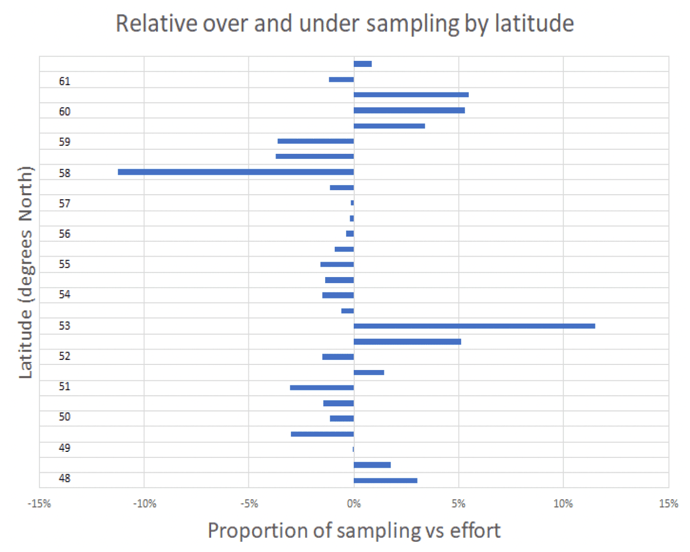
Figure 2 indicates that there is some systematic spatial bias in the sampling data through relative over-sampling at higher latitudes (60^o – 62^o N, roughly the latitude of the Shetland Isles) and at some mid latitudes (clustered around 53^o N, roughly the latitude of west Ireland) but relative under-sampling between 54^o and 59^o N (roughly northwest Ireland to the Scottish Western Isles). In part at least, this is explained by the fact that only about 200 hauls have been sampled, and hauls are autocorrelated within trips, meaning that sampling tended to occur in clustered regions within the full range of the fishery. Only by increasing sampling coverage levels and by specifically targeting sampling into specific areas would sampling ensure better representation across a wider range of latitudes. However, planning sampling in a fishery that ranges unpredictably over an area from the northern Bay of Biscay to the northern North Sea is challenging. Vessels tend to move fishing grounds within and between years to follow the concentrations of their target species, and potentially for other operational reasons. This means that it is difficult to focus sampling effort precisely on specific locations within the full fishery range in a way that would ensure more representative sampling distribution.

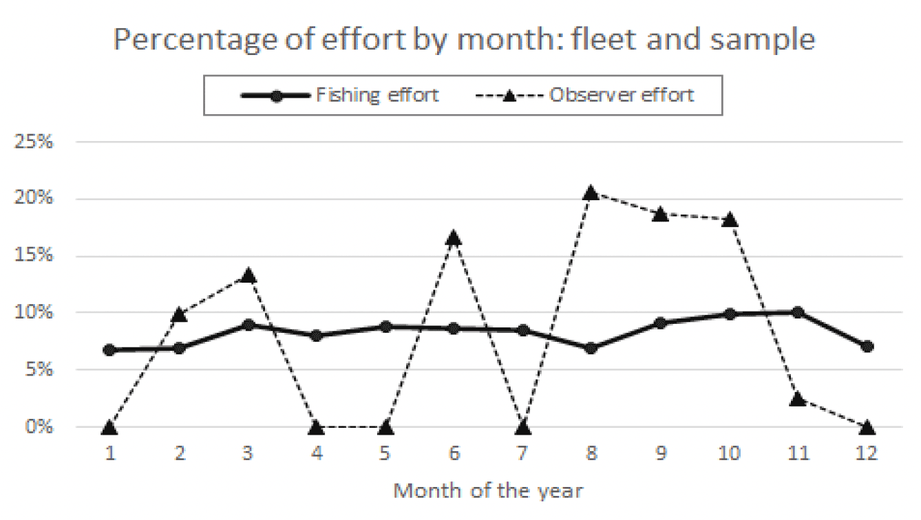
Ideally, intra-annual sampling levels would reasonably reflect fishing effort levels across the year. Figure 3 shows how observer sampling effort (orange line) was distributed by month, compared with fleet effort (blue line) by month over the ten-year period (2010 to 2019). Monthly fishing effort is more stable than monthly sampling effort and sampling does not closely represent the pattern of intra-annual fleet effort. Sampling levels were higher in the summer and early autumn months, and clear gaps are evident in December-January, April-May and July.

2.3 Modelling covariates

The data were analysed in a regression framework with the variation in bycatch per haul considered as a function of a variety of input variables. Because of the features of the data, namely the distributional properties and most especially the infrequency of bycatch, two distinct regression methods were considered: Generalized Additive Mixed Models (GAMMs, Wood 2017) and zero-inflated models. Neither approach was perfect for this data but the results from both analyses are presented. Geographic and vessel-based variables were considered.

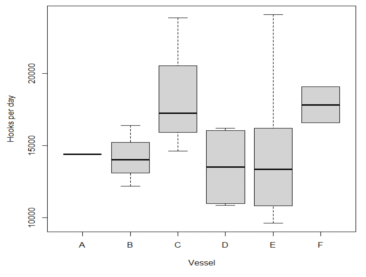
The data analysed consisted of individual hauls (n = 201) as the primary sampling unit. Hauls are undertaken on specific trips by a specific vessel, which in turn exhibit some degree of geographic clustering within ICES rectangles. Trips were also often spread over more than one (but usually adjacent) ICES rectangle. Some vessels consistently used fewer hooks per day than others (Figure 4). In statistical terms this is described as: hauls nested within trips and trips nested within vessels. Observed bycatch events are statistically quite rare implying a non-normal distribution of the data.

Given the data constraints (i.e., many zeros and a hierarchical data structure) the data were initially modelled in two ways. First as GAMMs, assuming a quasi-Poisson or negative-binomial distribution of the error to account for the potential correlation in the data and its hierarchical nature. Secondly, zero-inflated models were also considered using the R library pscl (Jackman 2020). In this case Poisson and negative binomial errors were considered. Model simple presence-absence using a binomial error structure was considered but because one output was estimates of total bycatch this was not feasible.

The dependent variable was the number of birds (of the relevant species) per haul. Sampling effort could be classified either by the number of hooks or total line length. Here we used the number of hooks as it was more directly related to the risk of bycatch.

Other available variables of potential influence on bycatch were Sea state, Day of year, Target species, Year, Latitude and Shot time measured as absolute time of day (Shottime) and as a proportion of the night length to account for light effects on bycatch, (Proptime). In addition, there were the broader effects of ICES Rectangle, Vessel and Trip.

Model selection was backwards using a P<0.05 inclusion criterion albeit with some modifications. P-value selection is more conservative than using the Akaike Information Criterion (AIC). P-values produce several scores per model and simple ranked model result tabulations, as often presented with AIC estimations, are not particularly informative using P-value based selection, so the model scores are not presented here.

The variables ICES rectangle, vessel and trip were all associated so it was difficult to tease these effects apart. The models were fitted first without these variables, then they were incorporated in the model and backwards model selection recommenced. Models with more than one of these variables produced unreliable fits. So ultimately trip alone was considered in the final models. However, it should be strongly stressed that Vessel, Trip and ICES rectangle are highly confounded in the dataset.

Models were fitted for northern fulmar and northern gannet, as only these two species had sufficiently high bycatch records to warrant an exploratory modelling approach.

2.3.1 Haul models for fulmars

Results are given for model selection undertaken on the two types of models: a GAMM with Trip as a random effect, and a zero inflated Poisson error model with Trip considered as a fixed effect. Both models are not quite ideal. The GAMM is less than ideal because there appears to be a residual structure in the error and the zero-inflated model is less than ideal because it cannot consider trip as a random effect at the cost of a few degrees of freedom and some correlation with the other variables. There was no evidence for unexplained temporal correlation in the residuals after the models had been fitted (see also Section 3.1).

GAMMs

The final model after model selection on the data considered as a GAMM is as follows.

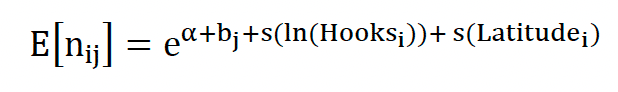
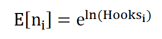
where represents the count in the ith datum, b_j is the effect associated with Trip factor j where Trip is a random effect (i.e., b_j is drawn from )) and Hooks and Latitude were covariates considered initially as thin plate spline smooths. A quasi-Poisson error structure was assumed with a log-link function.

The smooth of hooks collapsed down to a linear effect i.e.

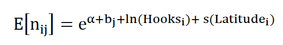
which makes logical sense if bycatch is simply proportional to the fishing effort as might be expected.

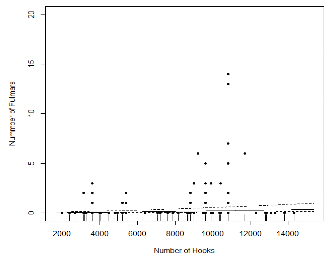
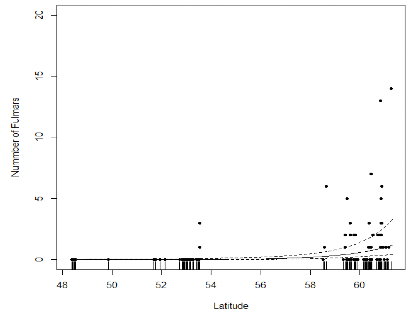
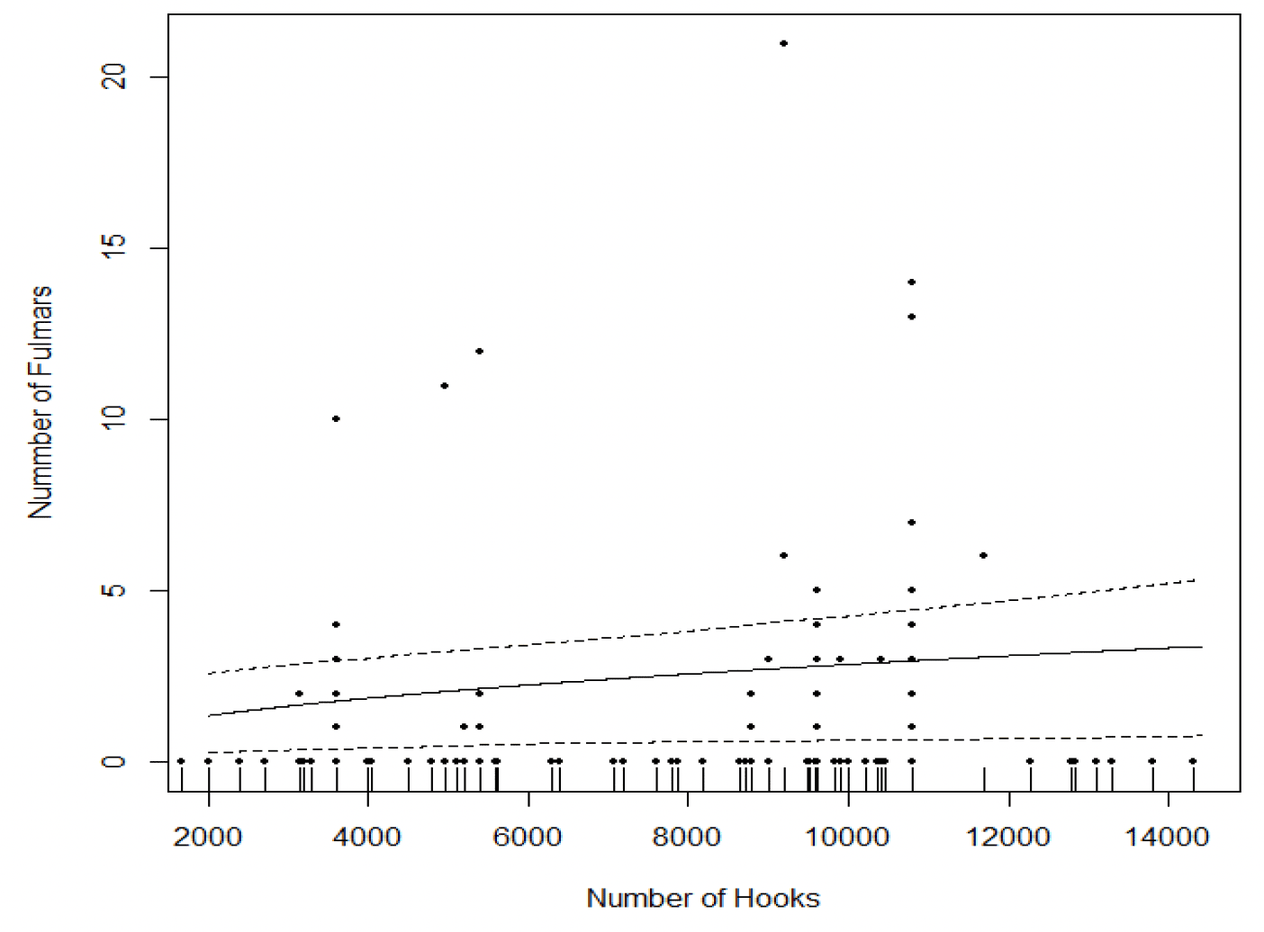
Figure 5 illustrates the Hooks effect from this latter model, which concludes that the effect of Hooks while detectable is negligible. Figure 6 shows the Latitude effect from this latter model which shows that more fulmars are caught at higher latitudes.

Zero-inflated models

Models with an assumed negative binomial error in the non-zero component were rejected by virtue of diagnostic plots and a boundary likelihood ratio test (after Hilbe, 2011). No fittable model involving Trip was found using backwards selection so forward selection with Trip was commenced based on the reduced set of variables found by the initial backwards selection. The best model here, consisted of Trip in the probability component (considered as a fixed factor) and number of ln (hooks) as a linear function in the count component of the model (Figure 5). The error was considered Poisson.

The count component was

The probability component is of form

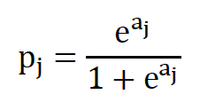
with α as the coefficient associated with every fixed level j of Trip.

No model that captured any effects on northern gannet bycatch could be found.

After considering the merits of the different models, the GAMM was used for estimating bycatch as these models seemed to be more robust.