Offshore renewable developments - developing marine mammal dynamic energy budget models: report
A report detailing the Dynamic Energy Budget (DEB) frameworks and their potential for integration into the iPCoD framework for harbour seal, grey seal, bottlenose dolphin, and minke whale (building on an existing DEB model for harbour porpoise to help improve marine mammal assessments for offshore renewable developments.
This document is part of a collection
10 Exploration of animal movement in iPCoD
This part of the study is separate from the DEB model development and the objective was to make a cursory exploration of the other key component impacting assessments of disturbance – the probability of exposure. Here we have explored how animal movement models may be utilised to refine the estimation of exposure histories for iPCoD
10.1 Why simulating movement is important
Currently in iPCoD, estimates of the number of animals of the species under consideration that may be disturbed, is an input number defined by the modeller. Furthermore, the model assumes that all individuals in a population are equally likely to be exposed to disturbance from a particular activity, or that only the members of a local population are likely to be exposed. The real-world situation is likely to be somewhere between these two extremes (see Keen et al. 2021). The use of movement simulation models is, therefore, required to generate more realistic exposure histories.
Here we demonstrate how movement models, for a single species, can be used to provide the kind of information required to improve realism and reduce conservatism in population level assessments.
The Disturbance Effects of Noise on the Harbour Porpoise Population in the North Sea (DEPONS) model is an individual-based model which can be used to predict annual movement patterns for a large number of “virtual” harbour porpoises in the North Sea and Inner Danish Waters. Below we demonstrate how we used DEPONS to estimate the number of days on which each virtual individual is likely to experience disturbance.
10.2 Simulating movement
We used the Inner Danish Waters harbour porpoise version of DEPONS as an example. We ran simulations for 200 individuals over 8 years: 3 years of burn-in period (the period the model needs to be run for before results can be robustly used) and 5 years of actual movement simulations. The duration of burn-in period was defined by observing population stability of the modelled individuals. Coordinates of each tracked individual were outputted in 30-minute time bins. DEPONS allows for tracking individuals from the beginning of the simulations to the death of these individuals during simulations. Individuals born during simulations are not tracked (see next paragraph for further explanation).
We then defined locations of two disturbance events with contrasting potential effect: ‘high’ (red, Figure 46) where the area of disturbance was superimposed on an observed high density region for porpoises, and ‘low’ (black, Figure 46), where the observed density of animals is low (Sveegaard et al. 2011). In both the high- and low-density regions, disturbance impact radii of 30, 45 and 60 km were superimposed.
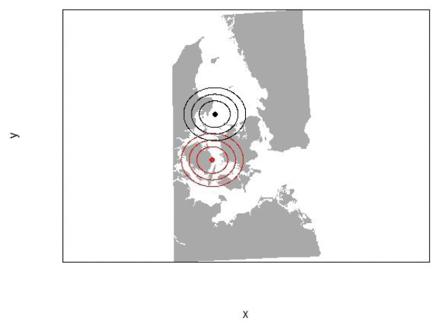
We then constructed a matrix to identify the number of hours per day each individual spends within any of these defined areas over the entire 5 years simulations (Figure 47).
This kind of matrix provides the kind of information conceptually required for transposing to iPCoD to inform analysis on harbour porpoises.
| ID | 1 | 2 | 3 | 4 | 5 | 6 | 7 | 8 | 9 | 10 | 11 | 12 | 13 | |
|---|---|---|---|---|---|---|---|---|---|---|---|---|---|---|
| 1 | 0_2010_1 | 24.0 | 24.0 | 13.0 | 18.0 | 8.0 | 0.0 | 0.0 | 0.0 | 0.0 | 0.0 | 0.0 | 0.0 | 0.0 |
| 2 | 0_2011_1 | 24.0 | 24.0 | 24.0 | 24.0 | 9.5 | 0.0 | 0.0 | 0.0 | 0.0 | 0.0 | 0.0 | 0.0 | 0.0 |
| 3 | 0_2012_1 | 0.0 | 0.0 | 0.0 | 0.0 | 0.0 | 0.0 | 0.0 | 0.0 | 0.0 | 0.0 | 0.0 | 0.0 | 0.0 |
| 4 | 0_2013_1 | 24.0 | 24.0 | 24.0 | 24.0 | 24.0 | 24.0 | 24.0 | 24.0 | 24.0 | 24.0 | 24.0 | 24.0 | 24.0 |
| 6 | 3_2010_1 | 24.0 | 24.0 | 24.0 | 24.0 | 24.0 | 9.5 | 23.5 | 24.0 | 24.0 | 24.0 | 24.0 | 24.0 | 14.5 |
| 7 | 3_2011_1 | 0.0 | 0.0 | 0.0 | 0.0 | 0.0 | 0.0 | 0.0 | 0.0 | 0.0 | 0.0 | 0.0 | 0.0 | 0.0 |
| 8 | 3_2012_1 | 0.0 | 0.0 | 0.0 | 0.0 | 0.0 | 0.0 | 0.0 | 0.0 | 0.0 | 0.0 | 0.0 | 0.0 | 0.0 |
| 9 | 3_2013_1 | 22.5 | 15.0 | 0.0 | 0.0 | 2.0 | 0.0 | 0.0 | 13.0 | 0.0 | 16.5 | 22.0 | 19.5 | 10.5 |
| 10 | 3_2014_1 | 2.0 | 24.0 | 16.5 | 24.0 | 17.5 | 21.0 | 24.0 | 3.0 | 11.0 | 24.0 | 24.0 | 24.0 | 24.0 |
| 11 | 4_2010_1 | 0.0 | 0.0 | 0.0 | 0.0 | 0.0 | 0.0 | 0.0 | 0.0 | 0.0 | 0.0 | 0.0 | 0.0 | 0.0 |
| 12 | 4_2011_1 | 24.0 | 24.0 | 11.5 | 16.0 | 24.0 | 24.0 | 17.0 | 0.0 | 0.0 | 0.0 | 0.0 | 1.0 | 17.0 |
This kind of approach could be explored further to allows other movement and exposure variables to be estimated:
- Individual and seasonal differences in the exposure history
- Frequency of occurrence within a disturbed area
- Inter-individual variability in duration and frequency of occurrence within the disturbed area.
All of these variables will sum to affect the realism of probability of exposure estimates.
10.2.1 Pitfalls
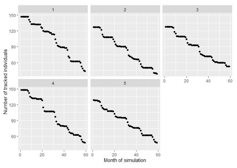
As mentioned above, DEPONS only allows for tracking of individuals which are created at the beginning of each simulation and the tracking stops when animals die. Individuals born after the start of the simulation are not tracked. DEPONS is also designed to simulate movement of so-called super-individuals: individuals which represent collectively larger number of individuals. Hence, DEPONS for Inner Danish Waters is designed to simulate maximum 200 ‘super-individuals’ and the results can then be extrapolated to the entire population in this area.
These above issues result in small number of individuals which can be tracked during actual simulations, after the end of burn-in period (Figure 48). As a consequence, the simulation of movement can only be performed for limited period of time – a maximum 10 years. After this period, there are very few or no animals which can be tracked by the model. This problem with low number of simulated and tracked individuals would be even more pronounced for simulations over large geographical space such as the North Sea.
Therefore, this is one of the limitations of this approach, that whilst it can provide the kind of information required to improve iPCoD simulations, it is limited by the sample size available (in terms of the number of animals that animals that can be tracked given simulation length and burn in period). This is a consideration that should be taken into account. But this approach demonstrates how movement models can be used to inform more realistic iPCoD simulations.
Contact
Email: ScotMER@gov.scot
There is a problem
Thanks for your feedback