Offshore renewable developments - developing marine mammal dynamic energy budget models: report
A report detailing the Dynamic Energy Budget (DEB) frameworks and their potential for integration into the iPCoD framework for harbour seal, grey seal, bottlenose dolphin, and minke whale (building on an existing DEB model for harbour porpoise to help improve marine mammal assessments for offshore renewable developments.
This document is part of a collection
8 Common minke whale DEB
8.1 Model parameters
Table 8 shows the parameter values used in most of the minke whale simulations described in this Chapter. Details of how these values were derived are outlined below.
| Parameter names | Code name | Value | Description | Source |
|---|---|---|---|---|
| Resource density | ||||
| R | Rmean | 2.315 | Annual mean resource density | See text |
| abeta | a_beta | 8.08 | Shape parameters of beta distribution defining stochasticity in resource density | See text |
| bbeta | b_beta | 24.25 | See text | |
| amplitude | 0.5 | Parameter defining the amplitude of seasonal variation in resource density | See text | |
| offset | 105 days | Parameter determining when during the year Rmean has its maximum value | See text | |
| Timing of life history events | ||||
| min_age | min_age | 6 years | Minimum age for reproduction | Christensen (1981) |
| mean_birthday | mean_birthday | 15 November | Mean pupping date for NE Atlantic stock | Hauksson et al (2011) |
| TP | Tp | 330 days | Gestation period | See text |
| TL | Tl | 150 days | Age at weaning (duration of lactation) | See text |
| TR | Tr | 150 days | Age at which calf’s resource foraging efficiency is 50% | See text |
| max_age | max_age | 50 years | Maximum age | |
| max_age_calf | 345 days | Maximum modelled age of calf | ||
| Reserves | ||||
| ρ | rho | 0.3 | Target body condition for adults | See text |
| θF | Theta_F | 0.2 | Relative cost of maintaining reserves | Hin et al. (2019) |
| Growth | ||||
| Lb | 247 cm | Length at birth | Hauksson et al. (2011) | |
| L0 | L0 | 415 cm | Length at weaning | Christensen (1981) |
| L∞ | Linf | 907 cm | Female maximum length | |
| b | b | - 0.000389 | Von Bertalanffy exponent | |
| ω1 | omega1 | 3.62x10⁻⁵ (kg/cm | Structural mass-length scaling constant | Hauksson et al. (2011) |
| ω2 | omega2 | 2.758 | Structural mass-length scaling exponent | |
| Energetic rates | ||||
| σM | Sigma_M | 2.5 | Field metabolic maintenance scalar | |
| σG | Sigma_G | 30 MJ/kg | Energetic cost per unit structural mass | Derived using the approach of Hin et al. (2019) |
| ε | epsi | 27.5 MJ/kg | Energy density of reserve tissue | Reilly et al. (1996) |
| ε- | epsi_minus | 24.75 MJ/kg | Catabolic efficiency of reserves conversion | |
| ε+ | epsi_plus | 34.03 MJ/kg | Anabolic efficiency of reserve conversion | |
| μs | mu_s | 0.2 | Starvation mortality scalar | Hin et al. (2019) |
| η | eta | 20 | Steepness of assimilation response | See text |
| ϒ | upsilon | 2.5 | Shape parameter for effect of age on resource foraging efficiency | See text |
| K | Kappa | 0 for calves & juveniles 0.5 for all other age classes | Proportion of the daily assimilated energy allocated to growth | See text |
| Pregnancy | ||||
| fert_success | fert_success | 0.9 | Probability that implantation will occur | Hauksson et al (2011) |
| Fneonate | F_neonate | Reserves required to cover costs of pregnancy and lactation | See text | |
| F_neo_multiplier | 0.9 | Fraction of F_neonate used as actual threshold | ||
| Lactation | ||||
| φL | phi_L | 5.4 | Lactation scalar | See text |
| σL | Sigma_L | 0.86 | Efficiency of conversion of mother’s reserves to calf tissue | Lockyer (1993) |
| TN | Tn | 135 days | Calf age at which female begins to reduce milk supply | See text |
| ξc | xi_c | 0.2 | Non-linearity in milk assimilation-calf age relation | See text |
| ξM | xi_m | 6 | Non-linearity in female body condition-milk provisioning relation | See text |
| Mortality | ||||
| foetal_mortality | foetal_mortality | 0.0 | Background foetal mortality | See text |
| α1 | alpha1 | 0.00045 | Coefficients of age-dependant mortality curve | Sinclair et al. (2020) |
| α2 | alpha2 | 0.943 x 10⁻⁴ | ||
| β1 | beta1 | 0.0004 | ||
| β2 | beta2 | 1.1 x 10⁻⁶ | ||
| ρS | rho_s | 0.1 | Starvation body condition threshold | See text |
| μs | mu_s | 0.2 | Starvation mortality scalar | See text |
| Disturbance | ||||
| Distdur | days.of.disturbance | Number of days on which disturbance occurs | See text for values | |
| Diststart | first_day | First day of disturbance period | See text for values | |
| Distend | Last_day | Last day of disturbance period | See text for values | |
| Disteffect | disturbance.effect | 0.25 | Reduction in resource density caused by disturbance | See text |
| AgeDist | age.affected | Age threshold defining which age class of simulated animals is affected by the disturbance | See text | |
8.1.1 Resources
Resource density (Rmean) Northeast Atlantic minke whales are believed to spend the summer on prey-rich feeding areas in northern latitudes and migrate south in winter to areas with much lower prey density. We modelled this variation by allowing resource density to vary seasonally following the sinusoidal curve shown in Figure 35. This predicts maximum resource density will occur around mid-July and that resource density may be effectively zero at some time during the winter.
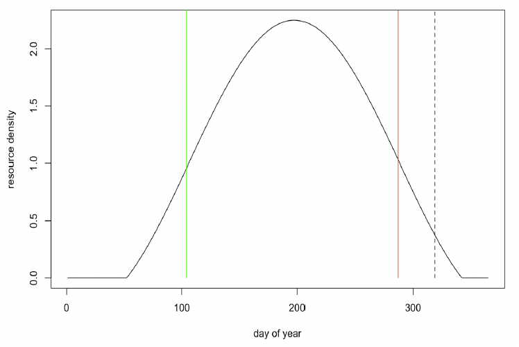
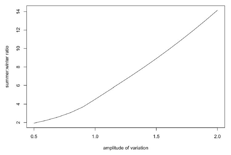
The duration of this period of zero resource density, and the difference in mean resource density between summer and winter, is determined by the amplitude of the sinusoidal variation, as shown in Figure 36.
Although it is often assumed that baleen whales do little if any feeding during the winter period, this is almost certainly not the case for Northeast Atlantic minke whales. The values for energy expenditure and energy acquisition in Table 1 of Nordøy et al. (1995) indicate that the energetic content of the reserves accumulated over the summer are only sufficient to cover field metabolic costs for 55 days of fasting in the case of adult females (mean length 8 m) and 64 days in the case of growing animals (mean length of 7 m). Therefore, these animals must be feeding for some of the time during the winter. We therefore set the amplitude of variation to a relatively low value (0.5, equivalent to a 2x difference in resource density between summer and winter) in our initial simulations.
In the original Hin et al. (2019) model resource density is assumed to be constant or to vary smoothly over the course of the year. However, in reality, the resource density encountered by an individual is likely to vary from day to day. This stochasticity in resource density can be modelled by multiplying Rmean for each day by a number drawn at random from a beta distribution with mean=1 and a 90% confidence interval of 0.5-1.5. Extreme values for this multiplier could be as low as 0.1 or as high as 2.4.
We assumed that calves encountered the same resource density as their mothers on each day during lactation.
8.1.2 Timing of life history events
Following Christensen (1981) we assumed that females had to be at least 7 m long before they could ovulate. The mean birthday for all calves was set at mid-November, as suggested by Hauksson et al. (2011).
Gestation period (TP) This is 10 months (~300 days) according to Perrin et al. (2018). However, a value of 330 days is more consistent with observed lengths at birth (see below).
Lactation period/age at weaning (TL) This is 5-6 months according to Perrin et al. (2018). However, Nordøy et al. (1995) and Jonsgård (1951) report that minke whales spend 6 months in Northeast Atlantic waters each year and that calves are not normally seen with these animals. Given the reported annual breeding cycle of minke whales, this suggests that lactation must last less than 6 months and we used a value of 150 days.
8.1.3 Reserves and growth
Reserve threshold (ρ) Nordøy et al. (1995) provided detailed information on changes in the mass and energy density of blubber, muscle and intra-abdominal fat for immature and adult Northeast Atlantic minke whales, from the time they arrive on the feeding grounds (around 14 April) until their departure 183 days later. We combined this with our calculations of the structural mass of animals of different lengths from the growth curve described below to estimate changes in body condition over the course of this period. The blubber mass and muscle mass of all individuals increased over the course of the summer, as did the energy density of these tissues (Nordøy et al. 1995). Nordøy et al. (1995) report that an 800 cm long whale increases its energy reserves by 151 MJ/day over the course of the summer, and we calculated that the average energy density of these tissues was 26 MJ/kg. The total energy accumulated in reserve tissue by an 800 cm long animal over the 183-day summer period is therefore equivalent to 1440 kg, resulting in a body condition of 0.28. However, some animals achieved a greater mass gain than this, and we therefore set ρ at 0.3.
Relative cost of maintaining reserves (ΘF) We were unable to find any published data that would allow a value specific to minke whales to be calculated for this parameter. We, therefore, suggest using the value of 0.2 assumed by Hin et al. (2019).
Structural length and structural mass (L0, L∞, ω1, ω2) A number of von Bertalanffy growth curves have been published for the Central and Northeast Atlantic minke whale stocks (Christensen 1981, Olsen and Sunde 2002, Hauksson et al. 2011), but the youngest animals in the samples used to fit these curves are usually at least 2 years old. None of the growth curves provide estimates of length at birth that are in the range 240-270 cm reported by Perrin et al. (2018), and only the Christensen (1981) growth curve is consistent with Jonsgård (1951) suggestion that length at weaning is about 450 cm.
Hauksson et al. (2011) fitted the following growth curve for minke whale foetuses, based on animals sampled at the Icelandic whaling station:
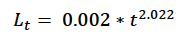
where t is the Julian days. Figure 2 of Christiansen et al. (2014) shows a similar pattern of foetal growth, probably because it is – at least in part - based on the same sample of animals. Hauksson et al’s (2011) curve predicts a length at birth of 204 cm if foetal growth begins on 1 January and gestation last 300 days, and 247 cm if gestation lasts 330 days. Only the latter value is consistent with the various estimates of length at birth for the Northeast Atlantic minke whale stock documented in Christensen (1981), supporting our assumption that TP = 330 days.
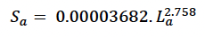
We estimated foetal weight at age using the following formula derived by Hauksson et al. (2011) from the same sample:
We assumed that growth in length was linear from birth to age TL (with a predicted length of 415 cm at this age) and then used Christensen (1981) growth curve
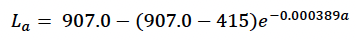
(re-parameterised to match the formulation used by Hin et al. 2019) from this age onwards. Structural mass at age (Sa) was calculated from La using Hauksson et al.’s (2011) formula for foetuses.
Modelling growth (Κ) The model developed by Hin et al. (2019) assumes that growth in length and core mass continues unabated, regardless of energy intake. This is clearly not the case in many marine mammals. We therefore assumed that growth may be reduced if energy intake is less than the combined costs of metabolism, growth and reproductive activities (pregnancy and lactation). We modelled these circumstances using a modification of the kappa rule, which is a fundamental component of classic DEB models (Kooijman 2010). We assumed that an individual will allocate a proportion of the assimilated energy (It) it acquires on a particular day to growth (including growth of the foetus, because this is treated as part of the female’s core mass), up to a maximum of (1-Κ).It. If this amount of energy is less than the energy required for growth, the growth rate of the female and her foetus is reduced accordingly. The balance of the energy intake is allocated to metabolism. If this is insufficient to cover all of the costs of metabolism, reserves must be metabolised. Values of Κ < 0.5 indicate that growth is prioritised over metabolism.
Following Christiansen et al. (2013) we set Κ to zero for immature animals, which are believed to prioritise growth above all else. Conversely, we assumed that nursing calves would prioritise reserves over growth, because adequate reserves are crucial to their survival in the post-weaning period. We experimented with a range of values of K for adult females.
8.1.4 Energetic rates
Field metabolic maintenance scalar (σM) Blix and Folkow (1995) estimated the average energy expenditure of 6 free-ranging, tagged minke whales to be 80 kJ/kg/day, based on their respiration rate. Folkow et al. (2000) used this value to calculate that a 5,900 kg adult minke whale would expend 472 MJ/day. This is equivalent to using a scalar of 1.7-2.5, depending on what assumptions are made about the values of ρ and ΘF. We used a value of 2.5 in both summer and winter to account for the potential increase in metabolic rate when animals are in warmer waters during the winter, as appears to be the case for baleen whales (Villegas-Amtmann et al. 2017).
Energetic cost per unit structural mass (σG) We calculated growth efficiency using the same approach as Hin et al. (2019), with a mass at birth of 144 kg (based on a length at birth of 247 cm) and an energy density of 3.8 MJ/kg for the tissue of minke whale foetuses estimated by Nordøy et al. (1995). This produced a value of 33 MJ/kg for σG.
Catabolic and anabolic efficiency of reserve conversion (ε-, ε+,) Nordøy et al. (1995) estimated that the energy density of minke whale blubber on arrival at the summer feeding grounds was 27.5 MJ/kg, very similar to the mean energy density of the tissues accumulated over the summer. Allowing for a 90% efficiency of catabolism, we assumed ε- = 24.75 MJ/kg.
In the absence of any direct measurements of ε+ for minke whales, we followed Hin et al. (2019) and used a value for ε+ that was 40% higher than ε- (i.e., 34.65 MJ/kg).
Steepness of assimilation response (η) We were unable to find any data in the literature that could be used to set a feasible range for this parameter. We explored the implications of values between 5 and 25 and found that predicted changes in body weight and reproductive success were relatively insensitive to the value of this parameter. We therefore carried out most simulations with a value of 20.
Effect of age on resource foraging efficiency (Υ, TR): We could find no information that could be used to estimate these parameters in the literature. Initially, we assumed that calves are 50% efficient at foraging when they are weaned.
8.1.5 Pregnancy
Pregnancy threshold (Fneonate): Jonsgård (1951) observed that most adult females on the feeding grounds were pregnant, suggesting that minke whales have a one-year reproductive cycle. Christiansen et al. (2014) observation that female minke whales on the Icelandic feeding grounds that were in poor condition (as measured by their blubber volume) had smaller foetuses suggests that females respond to reduced energy intake in summer by reducing their investment in their offspring rather than by terminating a pregnancy. However, there is a high risk of starvation-related mortality if females attempt to complete lactation when they have insufficient energy reserves. We, therefore, experimented with a range of value for Fneonate on day 300 of pregnancy. This is equivalent to 15 October in the Northeast Atlantic and represents the date at which most females leave the feeding grounds. We calculated the amount of energy a female would require to complete her pregnancy and provide her calf with 100% of its energy requirements during the lactation period. We then examined the consequences of setting a threshold for continuing a pregnancy that was a fraction of this value. Female fitness, measured by lifetime reproductive success at a particular value of Rmean, increased as the magnitude of the threshold was increased from 0.8* Fneonate to 0.9* Fneonate, but there was little increase beyond this value. We, therefore, carried out all subsequent simulations with a threshold of 0.9* Fneonate.
Probability that implantation will occur (fert_success) The probability of successful implantation was set at 0.88 based on the ovulation rate reported by Hauksson et al. (2011).
8.1.6 Lactation
Efficiency of conversion of mother's reserves to calf/pup tissue (σL): In the absence of any direct measurements of the relevant efficiencies for minke whales, we suggest using the value of 0.86 that was used by Hin et al. (2019).
Effect of calf/pup age on milk assimilation (ξC, TN): It is generally assumed that resource density is low on the breeding grounds and that females will provide almost all of their calves’ energy requirements up to the age at weaning. We therefore set TC = 0.9*TL.
Effect of female body condition on milk provisioning (ξM) Because calves are weaned on the breeding grounds or during migration to the summer feeding grounds, lactating females that are in poor condition at this time will be close to the starvation threshold and may struggle to recover their depleted reserves. We therefore assumed a “conservative” strategy in which females began reducing milk supply relatively rapidly as their condition declined (i.e., a value of ξM ≥ 5, see Figure 6). Values of ξM > 5 resulted in increased levels of adult female mortality, without any obvious improvement in fitness. We therefore carried out all simulations with ξM = 5.
Lactation scalar (ΦL) We calculated the total costs of calf growth and calf metabolism during the period when females are assumed to be providing 100% of their calf’s energy needs and assumed that the calf’s body condition was close to ρ throughout this period.
8.1.7 Mortality
Age-dependent mortality rate We followed the approach used by Hin et al. (2019) and estimated changes in the probability of survival with age using the method developed by Barlow & Boveng (1991). The following function describing the variation in daily survival with age:
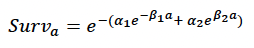
where a is age in days, was fitted to the annual age-specific minke whale survival rates from Taylor et al. (2007). We used a maximum age of 50 years, based on the fact that the oldest female in a sample of 288 whales examined by Hauksson et al. (2011) was 42 years old and that Taylor et al. (2007) propose a maximum age of 51 years. The resulting fitted values were:
α1 = 0.00045
β1 = 0.0004
α2 = 0.943 x 10⁻⁴
β2 = 1.1 x 10⁻⁶
Figure 37 shows the fitted curve. Combined with a pregnancy rate of 0.9, these survival rates generate a population growth rate of 1.05. The life expectancy of each simulated female was calculated by choosing a random number between 0 and 1 and determining the age in days at which cumulative survival equalled this value.
Foetal mortality In the absence of any empirical information on foetal mortality, this parameter was assumed to be zero.
Starvation body condition threshold (ρs) We combined information on body composition from Nordøy et al. (1995) with estimates of structural body mass at different lengths from our growth to estimate that the mean body condition of sub-adult and adult animals on arrival at the feeding grounds was 0.12, based on the ratio of blubber mass to total mass. Adult females arriving on the feeding grounds will have just finished lactation and migration from their breeding grounds, so a body condition of 0.12 should represent a typical minimum level in their annual cycle. This suggests that 0.1 is an appropriate value for ρs.
Starvation-induced mortality rate (μs) No empirical information that could provide a species-specific value of this parameter for minke whales is available. As a starting point for exploratory modelling, we used the value of 0.2 proposed by Hin et al. (2019).
8.2 Model results – pattern-oriented modelling
We used three additional sources of information to investigate the performance of the minke whale DEB model.
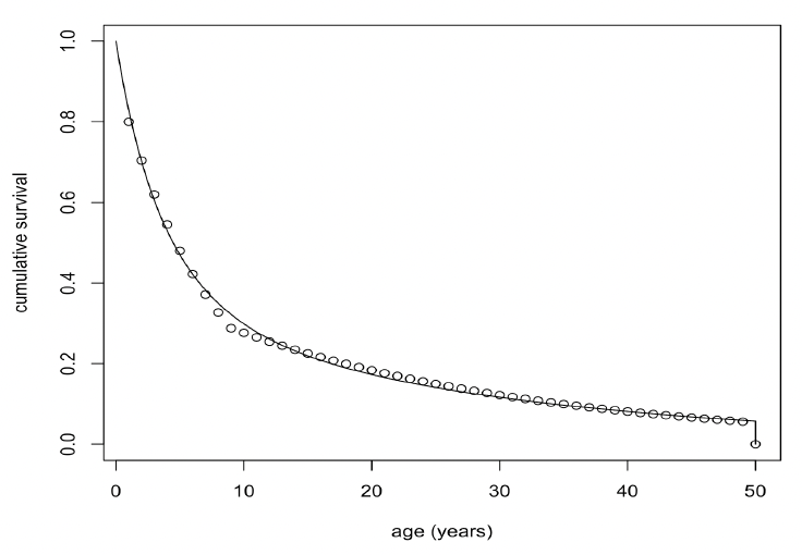
Nordøy et al. (1995) documented the relationship between female length and blubber mass in animals killed at the start (average catch date 19 May) and end (average catch date 9 September) of the Norwegian whaling season and found that the slope of the regression relating these two variables was higher in animals taken at the beginning of the whaling season; the DEB model generated similar outputs (Figure 38).
Christiansen et al. (2013) found that the total blubber volume of pregnant and mature female minke whales killed in the Icelandic whale hunt increased over the course of the whaling season, while the blubber volume of immature animals did not (Figure 39). Again, the DEB model predicted very similar changes.
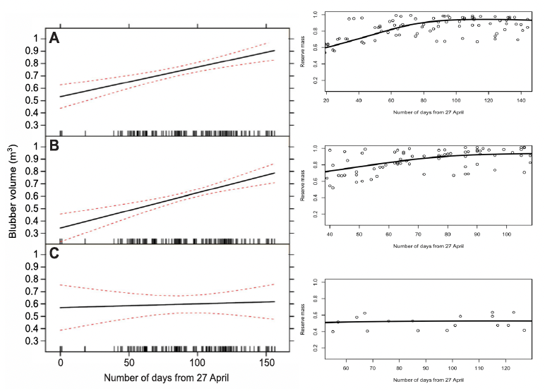 DEB model. As described in the text above.">
Christiansen et al. (2014) used the same information to show that pregnant females that were in poor body condition (with a lower-than-expected blubber volume at a particular date in the whaling season) had foetuses that were substantially shorter than females that were in average or good condition. We were unable to duplicate this relationship in the DEB model, partly because all simulated females within a particular simulation experienced exactly the same resource density at a particular time of year, and therefore had similar blubber mass. Reducing Rmean to simulate the effects of low resource density for all whales did result in slightly smaller foetuses, but the main effect was to increase starvation-related mortality of females during the lactation period. This suggests that Christiansen et al.’s (2014) observations were the result of short-term variations in energy intake among individuals within a year, a process we were unable to capture in the DEB model.
8.3 Simulating the effect of disturbance
We assumed that common minke whales would only experience disturbance in UK waters during the summer months. Although there is some information on the response of minke whales to military sonars (Kvadsheim et al. 2017, Durbach et al. 2021), there is no equivalent information on the response of minke whales to piling noise. We initially assumed a similar response to that observed in harbour porpoises, with a 25% reduction in foraging efficiency on days when animals were exposed to this kind of noise, but disturbance on this scale had very little effect on vital rates. The following results assume that disturbance results in a 50% reduction in foraging efficiency.
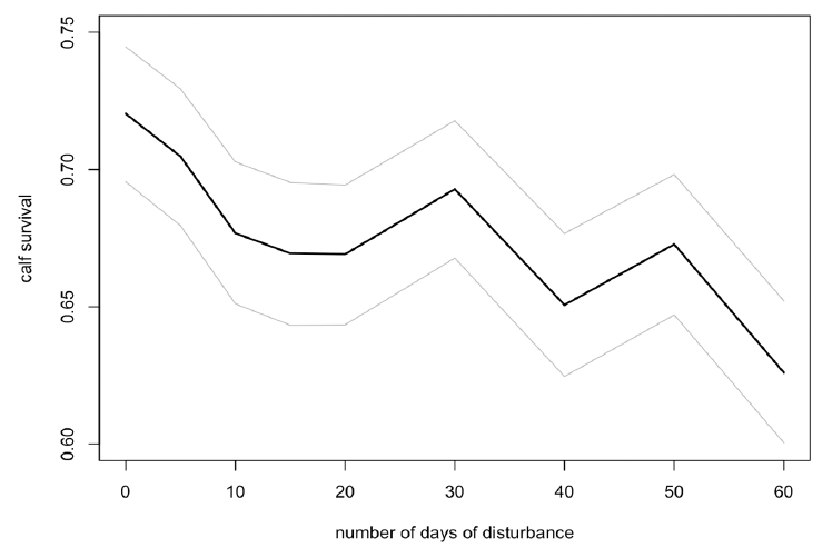
Disturbance had a small effect on calf survival if it was spread randomly across the entire summer (Figure 40), but no effect if it was confined to the first three months of the summer (mid-April to mid-July).
However, there was a greater effect on calf survival if disturbance was confined to the period mid-July to mid-October (Figure 41). The effect was greatest on the calves of younger females (<25 years old), whose survival was reduced by 80%.
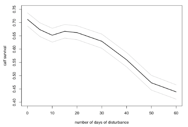
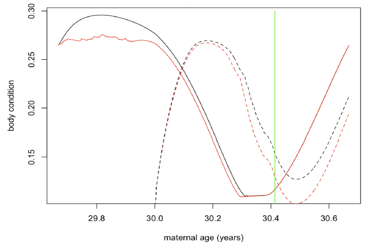
Figure 42 shows the changes in maternal and calf condition that cause this additional calf mortality.
Contact
Email: ScotMER@gov.scot
There is a problem
Thanks for your feedback