Offshore renewable developments - developing marine mammal dynamic energy budget models: report
A report detailing the Dynamic Energy Budget (DEB) frameworks and their potential for integration into the iPCoD framework for harbour seal, grey seal, bottlenose dolphin, and minke whale (building on an existing DEB model for harbour porpoise to help improve marine mammal assessments for offshore renewable developments.
This document is part of a collection
9 Accounting for uncertainty in DEB models
9.1 Sources of uncertainty
The DEB models developed in this report require values for more than 30 parameters and it is important that model outputs take account of the uncertainties that are associated with these values. In many cases (e.g., the parameters that determine mass at age, and age-specific survival) these values are estimated from empirical data and the uncertainty associated with them is primarily a result of measurement and sampling error, and among-individual variation. There are standard procedures for quantifying the effects of these uncertainties, such as sampling at random from the statistical distributions associated with the parameter estimates, and we have not investigated these sources of uncertainty in this report. However, it would be valuable to investigate the extent to which the uncertainty is a result of among-individual variation. If most of the uncertainty is due to individual variation, different resampled values should be applied to individuals rather than all members of the simulated population and this is likely to affect the sensitivity of model outputs to this uncertainty.
Although estimates of FMR are available for many species, these estimates are often highly variable within a species and we did attempt to find a reliable approach to account for this uncertainty (see next sections). A similar issue will arise if no empirical estimate of a potentially measurable parameter is available for the species that is being modelled and values have to be “borrowed” from other, better studied species that have a similar life history strategy.
Finally, there is a suite of parameters that control the rules that determine the decisions made by simulated individuals about how to allocate surplus assimilated energy to growth or reserves, how foraging efficiency increases with age, when females should abandon a pregnancy or calf because their reserves are too small, and how reserves levels affect the risk of individual mortality. It is very difficult (and sometimes impossible) to determine the rules (if any) that free-living animals are actually implementing. We intended to build on an Office of Naval Research (ONR) supported effort on “Advancing PCOD efforts through a marine mammal bioenergetics workshop” which aimed to review the current state of knowledge of both modelling (building on Pirotta et al. 2018a) and data needs to support the development of bioenergetic models via a series of mini reviews of key bioenergetic topics (metabolic rates, reproductive energetics, growth and energy intake). The outputs of that workshop will appear in the Conservation Physiology Special Issue in 2022.
It became clear from our sensitivity analyses of the different DEB models that there are strong interactions between some of the subjective parameters which would make it very difficult for experts to assess the likely biological implications of particular combinations of parameter values. With the above points in mind, we chose to use Approximate Bayesian computation rather than expert elicitation. This allowed us to identify biologically plausible combinations of values for these parameters that are consistent with what is known about the population characteristics of the species being modelled. In the next sections, we use this approach to identify a plausible parameter space for the grey seal DEB model, and sample from this space to investigate the effects of uncertainty in these parameters on the predicted effects of disturbance on one vital rate (pup survival).
9.2 Quantifying uncertainty
We applied Approximate Bayesian Computation (ABC) parameterisation to establish plausible distributions for each of the parameters listed in Table 9. The ABC technique consist in (i) simulating the model a very large number of times with parameter values drawn from prior distribution, (ii) comparing the simulation outputs to observational data and (iii) retaining those parameter combinations that were consistent with observations (Jabot et al. 2013).
The potential range of values for each of the parameters listed in Table 9 is vast and simply sampling from these ranges would result in an impossible computational task. We therefore did a preliminary manual screening of potential values to identify those that resulted in relatively high values of mean lifetime reproductive success (a measure of individual fitness) at a particular value of Rmean. We reasoned that genotypes that resulted in traits that replicated the rules implied by those parameter combinations would have a strong selective advantage and would rapidly dominate the population. The resulting plausible ranges were used to define the limits of the uniform prior distributions for the parameters shown in Table 9.
| Parameter | Description | Prior distribution |
|---|---|---|
| K (Kappa) | Proportion of surplus assimilated energy allocated to growth | Uniform(0.6, 0.9) |
| ϒ (upsilon) | Shape parameter for effect of age on resource foraging efficiency | Uniform(1.4, 1.75) |
| TR | Age at which calf’s resource foraging efficiency is 50% | Uniform(70, 120) |
| μs (Mu_s) | Starvation mortality scalar | Uniform(0.1, 0.3) |
| σM (sigma_M) | Field Metabolic Rate scalar | Uniform(2, 3) |
| Rmean | Mean resource density | Uniform(1.3, 2.4) |
| decision_day | Day of pregnancy when female decides whether or not to continue | Uniform(160, 200) |
| ρS (rho_s) | Starvation body condition threshold | Uniform(0.05, 0.15) |
We applied ABC in a stepwise fashion. In the first step we ran 20,000 simulations, each involving 1500 females (which we had previously established as the minimum number of simulated animals necessary to obtain a reliable and unbiased estimate of mean lifetime reproductive output and population growth rate) using the prior distributions listed in Table 10. The main aim of this first step was to identify parameters which are strongly correlated. Once correlation between parameters was established, we ran an additional 60,000 simulations using the same prior distribution for all non-correlated parameters and drawing values of the correlated parameters from the relationship established in step 1. We developed a set of rejection criteria based on available estimates of the population characteristics of UK grey seal populations, as described in Thomas et al. (2019) and Smout et al. (2019).
| Pattern | Rejection criteria | Used in step |
|---|---|---|
| Annual population growth rate | <0.985 or >1.035 | 1 & 2 |
| Median birth rate | > 0.8 | 1 & 2 |
| Female starvation mortality | < 0.2 | 1 & 2 |
| Pup survival | <0.14 or >0.22 | 2 |
The first step revealed that there is a strong correlation between Rmean and sigma_M (Figure 43) and the established relationship between these two parameters was used in the second step.
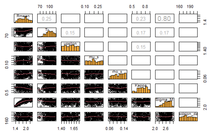
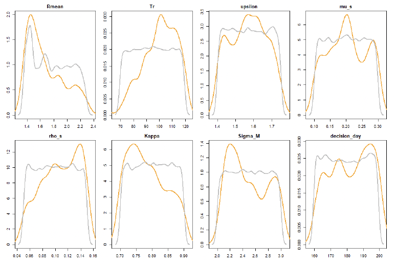
The 60,000 simulations in step 2, resulted in 519 parameter combinations fulfilling all the criteria listed in Table 10. The prior and posterior distribution of these parameters is shown in Figure 44. These 519 combinations were then used to investigate the effect of uncertainty on the predicted relationship between disturbance and vital rates.
9.3 Effects of uncertainty on the predicted relationship between disturbance and vital rates.
Figure 45 shows the predicted effects of disturbance on calf survival and birth rate for 10-year-old and 21-year-old female grey seals using 100 parameter combinations randomly selected, without replacement from the 519 combinations generated by the ABC analysis. A total of 1500 were simulated for each combination of parameter values and number of days of disturbance, and disturbance was assumed to result in a 25% reduction in foraging efficiency (equivalent to a cessation of foraging of 6 hours during the day on which disturbance occurred). Few studies have explored this directly. Czapanskiy et al. (2021) describes a 1-hour cessation of foraging to be mild, 2 hours to be moderate and 8 hours to be an extreme response. Disturbances were scheduled to occur on random days within the period from implantation until the female decided whether or not to continue the pregnancy. For seals breeding at the Farne Islands, this is the period from late March to the end of August, which is when piling for offshore wind farms in the North Sea is most likely to occur.
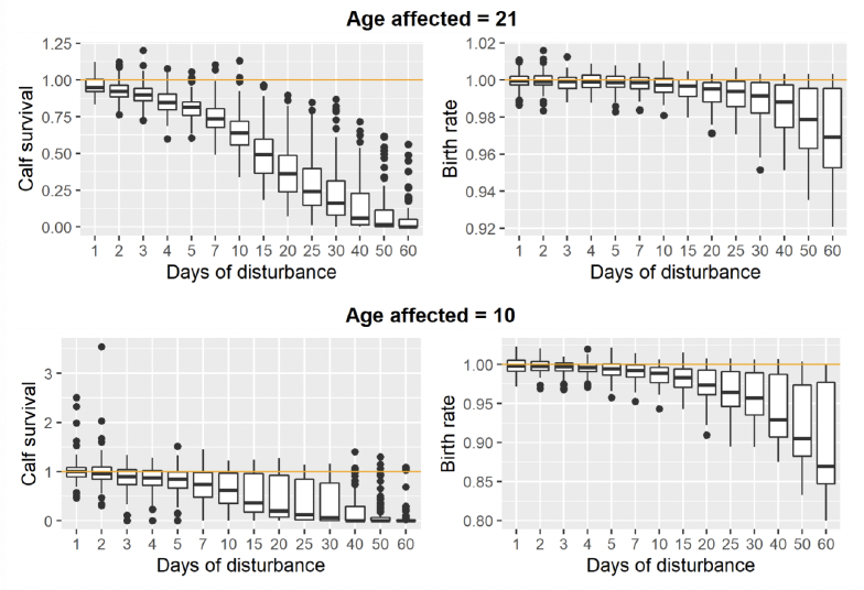
In principle, relationships such as those used to produce Figure 45 can be incorporated into iPCoD as an alternative to the “virtual expert” relationships derived from expert elicitation that are currently used. However, it is critical to note that the effect of disturbance (assumed to be 6 hours lost foraging here for indicative purposes only) would need to be carefully considered as relationships will vary depending on the selection of this value.
Some changes to the iPCoD code would be required to take account of the fact that the effects of disturbance predicted by the DEB model are different at different times of year. However, iPCoD requires the user to input a calendar of disturbance events and it records the disturbance history of each simulated individual exposed to these events, so these histories can readily be divided into appropriate sensitive periods.
Contact
Email: ScotMER@gov.scot
There is a problem
Thanks for your feedback