Scottish Marine and Freshwater Science Vol 6 No 6: Development of a Model for Predicting Large Scale Spatio-Temporal Variability in Juvenile Fish Abundance from Electrofishing Data

Covariates

Covariates were obtained for each sampling location. The selection of covariates was informed by previous habitat modelling studies (Fausch, 1988; Niemela et al., 2000; Wyatt 2005; SNIFFER, 2011) or relationships between covariates and processes that influence abundance, or capture probability. For example Altitude influences river temperature and in turn potentially affects fish productivity and capture probability, whereas Organisation may be expected to affect capture probability through differences in equipment or personnel, but should not affect fish productivity directly.

The continuous spatial covariates were: Upstream Catchment Area ( UCA), Altitude, river network Distance to Sea ( DS), Gradient, Channel Width (Width), landuse (see below for details). Data provider (Organisation) was included because of possible effects on catch probability. Hydrometric Area ( HA) was included as a large scale spatial covariate. Catchment was also included to allow for finer scale deviation from regional trends. Options were also explored for including river network data that described spatial relationships between sampling points, hereafter referred to as River Connectivity ( RC). Year and Day of Year (DoY) were included to allow for temporal variability. The location of sites above or below fish barriers was characterised to allow further data refinement depending on the species considered.

Before calculating spatial covariates it was necessary to assign (snap) sampling sites to a spatial dataset that represents Scotland's rivers. In this case the SEPA rivers dataset was chosen to provide the base mapping, where rivers are represented by a series of connected line features. In the case of MSS electrofishing data, a manual check of locational accuracy was performed, but this was not possible for externally sourced data. The resulting layer of snapped sites was used to obtain spatial covariates, the details of which are described below. All GIS analyses were performed in ESRI ArcGIS version 10 unless otherwise stated.

The selected covariates can be broadly assigned to four groups (1) spatial covariates (Hydrometric Area, Catchment and River Connectivity), (2) habitat covariates (Altitude, Upstream Catchment Area, Distance to Sea, Gradient, Landuse and Channel Width (3) sampling covariates (Organisation) (4) temporal covariates (Year and Day of Year).

1. Spatial Covariates

Hydrometric Area

SEPA hydrometric areas are administrative regions including a single large catchment or a number of contiguous smaller catchments with similar topographical characteristics (Marsh and Hannaford, 2008). They represent an intermediate spatial scale useful for modelling correlated regional variability in fish abundance. All Sites were attributed to a hydrometric area using the 'overlay' function in the R package rgdal and the SEPA hydrometric area polygons shapefile. In this report, HA was a regional identifier that links to additional information on connectedness to other regions (see 'Adding Regional Smoothers' in the Software section).

Catchment

All sampling points were allocated to a SEPA Baseline or Coastal river catchment. SEPA baseline rivers are only those catchments with an area of >10km2. Catchments were too numerous for describing large scale regional variability in fish abundance, but were useful for describing finer scale deviations from regional trends.

River Connectivity

To describe spatial variation on a network, it is only necessary to know the connectedness of sampling locations and confluences. There is therefore considerable redundant information in the full river network dataset. The R package igraph (an R package for analysis of mathematical graphs), describes the connectedness of sampling points on a river network and the function 'reduceNetwork' reduces the information to a manageable size (see 'Adding a River Network Smoother' in the Software section). The River Connectivity covariate is essentially an identifier for a node on the river network that links to additional information on connectedness to other nodes.

2. Habitat Covariates

Altitude

A National Digital Terrain Model ( DTM) provided by Centre for Ecology and Hydrology ( CEH), was used to derive both altitude and slope (see below) for each sampling point. Altitude was obtained directly from the DTM using the 'Extract Values to Points' function.

Upstream Catchment Area

Upstream catchment area was obtained using the accumulation grid dataset provided by the CEH and the 'Raster Calculator' tools within spatial analyst. The latter calculates the number and size of upstream cells contributing to each cell in the CEH DTM. In common with the altitude and slope extractions, values for upstream areas were obtained using the 'Extract Values to Points' function from the resulting raster file.

Distance to Sea (along river network)

Rivers within the SEPA rivers dataset are split into connected line segments of known lengths and organised so that it is possible to take a point on the river and measure its route to the mouth. The distance to mouth was calculated for each sampling location using the 'Locate Features Along Routes' tool within 'Linear Referencing'.

Gradient

A slope raster was created within the 'Spatial Analyst' toolbox using the CEH DTM. For each 50m cell, the 'Slope' tool calculates the maximum difference in height between that cell and its surrounding neighbours and calculates the maximum gradient in degrees. Using the new raster, slope values were then obtained again using the 'Extract Values to Points' function.

Landuse

Metrics of land use and channel width were obtained from the Ordnance Survey MasterMap dataset. An automated script (within the 'select' option) was used to group polygons into land use themes, including inland water (rivers and lochs), Marsh, Urban, Mixed Woodland, Deciduous Woodland, Conifer Woodland and Other. The 'buffer' tool was then used to create 50m diameter circular polygons around each sampling location from which percentage landuse characteristics were obtained having removed the area associated with inland water polygons. For each theme, the 'intersect' command was used to ascertain the overlap with the site buffer. The 'dissolve' option, which aggregates features ( i.e. unique site name) based on specified attributes ( i.e., total area of specific land use type) was then used to merge the multiple theme polygons. The area for which riparian landuse was characterised varied depending on river width from a maximum of 1965m2 to a minimum of 85m2. Only 2.5% of sites were characterised by land areas of <1000m2. As such, although with limitations, this approach provided a useful metric of "local landuse" in the vicinity of the sampling location.

Channel Width

A similar approach to that used to determine landuse was used to approximate mean channel Width from the perimeter and area of inland water polygons within the buffer using the following equation:

This approximation is increasingly accurate for polygons with a more rectangular shape, but nevertheless should identify major differences in channel width where this can vary over > 2 orders of magnitude. Unfortunately OS MasterMap defines all waterbodies less than 1m (urban areas) or 2m (rural areas) in width as line features. This results in areas and perimeters of 0. A manual correction was therefore applied to these cases with fixed values of 1.0 m where land use type was predominantly urban or 2.0 m elsewhere.

3. Sampling Covariates

Organisation

All data were assigned an organisation. There was some spatial structuring in the data from fisheries trusts. However, data provided by MSS and SEPA was geographically spread, and some trusts generated data in other trust areas thereby reducing the potential for confounding the effects of organisation and space (which was also represented by hydrometric area).

Sources of Error in Covariates

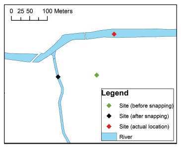
A number of technical problems were identified while generating spatial covariates. At the most basic level, sites often had incorrect grid references which placed them in the wrong catchments or even in the sea. Fortunately, these problems were straight forward to identify and the data could be omitted. Less obvious problems arose where site locations were recorded with low precision or lesser degrees of inaccuracy. Under such circumstances sites could be snapped to the wrong river line ( Fig. 3) with serious consequences for the estimation of certain covariates. These issues were possible to correct where the electrofishing locations were known, but not where data was provided by other organisations.

Figure 3 Example showing the consequences of low precision or inaccurate measurements of Site location. In this example the recorded site location was not on a river. Snapping to the nearest river places the Site on a tributary rather than the main-stem river where it was actually located. Based on digital spatial data licensed from the Centre for Ecology and Hydrology, © NERC. © Crown copyright. Licence 100024655.

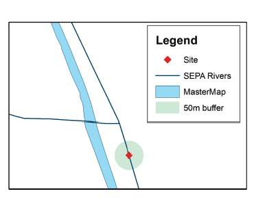
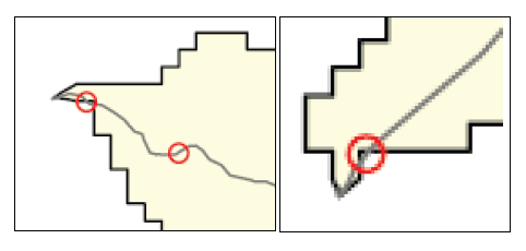
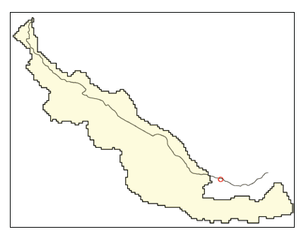
Problems also arose where spatial data had been captured at different resolutions and were therefore not completely coherent. For example, the SEPA rivers line dataset (derived from the CEH rivers dataset) was not always spatially coherent with the OS MasterMap polygon dataset. This caused problems because it was necessary to snap site locations to the SEPA rivers, but then to estimate river widths from MasterMap. Where the two were not coherent this could result in erroneous estimates of channel width or other landuse characteristics ( Fig. 4). Similarly, there were circumstances where sites could be incorrectly allocated to catchments because of the spatial resolution and precision of catchment boundaries ( Fig. 5) or due to other unknown errors ( Fig. 6). However, these issues were resolved by identifying the river on which points were located rather than the specific location.

Figure 4 Example of circumstances where SEPA rivers line features and MasterMap polygons were spatially incoherent. In this example the buffer does not contain any inland waters polygons. As such this would result in an estimated mean channel width of zero. Based on digital spatial data licensed from the Centre for Ecology and Hydrology, © NERC. © Crown copyright. Licence 100024655.

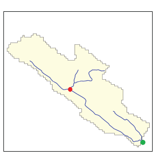
Finally, there were circumstances where the SEPA rivers line dataset contained connectivity errors that needed to be corrected ( e.g., Fig. 7). Each river segment in the dataset has a 'from' and a 'to' node which identify connections to other segments and flow direction. River sources have a 'from' node that does not reference to other valid nodes. Similarly river mouths have a 'to' node specified in the same way. Problems arise where the 'to' and 'from' nodes are misspecified so they are connected to distant rivers, flow in the wrong direction or appear as breaks in the network. Problems were identified by visually inspecting plots of the routes between sampling sites and river mouths. In practice, resolution of these problems was achieved by re-specification of all river node names in the SEPA rivers dataset using their unique latitude and longitude combination.

Figure 5 Examples of differences in spatial resolution resulting in incorrect allocation of Sites to Catchments. Red circles indicate sampling sites, black lines catchment boundaries and grey lines, rivers. Based on digital spatial data licensed from the Centre for Ecology and Hydrology, © NERC.

Figure 6 Examples where a SEPA river line runs outside of the catchment polygon. The sample point (red dot) lies on the river (grey line) but is outside the catchment boundary polygon (black line, shaded). Based on digital spatial data licensed from the Centre for Ecology and Hydrology, © NERC.

Figure 7 Example of a false river mouth due to un-connected river segments. The true river mouth (green circle) is in the south east, but there is an extra river mouth (red circle) assumed. © Crown copyright. Licence 100024655. Based on digital spatial data licensed from Centre for Ecology and Hydrology, © NERC.