Marine piling - energy conversion factors in underwater radiated sound: review
A report which investigates the Energy Conversion Factor (ECF) method and provides recommendations regarding the modelling approaches for impact piling as used in environmental impact assessments (EIA) in Scottish Waters.
This document is part of a collection
2. Review of Current Practices
This section provides a review of the ECF as it has been used in certain acoustic modelling projects providing predictions of the radiated sound field from marine piling operations. The section is divided based on two distinct aspects of the modelling. First, we look at how the source is defined in these projects, and the shortcomings of current methods. Second, we pay closer attention to how the propagation of sound is modelled.
2.1. The Pile as a Sound Source
The most common general method for predicting underwater sound levels resulting from an audible process in the water is to start with a source level and calculate the propagation loss, i.e., attenuation of sound, between the source and the receiver. Consequently, based on this method, a reasonable prediction of the source level is required.
It must be made clear at this stage that in the case of impact piling there is no source level for reasons that are discussed later in this section; it would be technically incorrect to refer to it as such. In this context, however, the pile is reproduced as a point source somewhere in the water column.
It is also valuable to note that there is a distinction between ‘source level’ and ‘energy source level’, with full definitions provided in ISO 18405:2017. The source level is related to the mean-square sound pressure of a statistically stationary sound source, i.e., one that is providing constant continuous sound, and thus is independent of time. The energy source level is based on the time-integrated squared sound pressure, and thus is a measure of the total sound energy within a set time interval. Given the nature of the piling pulse, it is more appropriate to use the energy source level over the source level.
Use of the “acoustic energy conversion efficiency” to convert to the “source level energy” of a pile driving strike is described by Farcas et al. (2018) in the following extract:
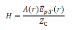
“The source level estimate for pile driving was calculated using an energy conversion model, whereby a proportion of the expected hammer energy is converted to acoustic energy:
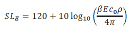
where is the hammer energy in joules, is the source level energy for a single strike at hammer energy , is the acoustic energy conversion efficiency, is the speed of sound in seawater in ms-1, and p is the density of seawater in kg m-3”
The source level (or energy source level) of an underwater sound source is defined in terms of its far-field sound pressure. From ISO 18405 (2017), the acoustic far field is the “spatial region in a uniform medium where the direct-path field amplitude, compensated for absorption loss, varies inversely with range”. In Section 2.1.1, we explain that the sound propagation from a driven pile does not fulfil the criterion for a far-field state as described above; as the driven pile has no far field it therefore has no source level (Ainslie et al. 2020). For other sound sources of potential interest, one can write a similar equation
Here, c0 and p0 are the sound speed and density of the medium, E is the input energy to the source (for an airgun this could be the potential energy stored in the compressed air; for a sonar pulse it could be the electrical energy used to drive the transducer), β and is the ECF.
As a pile driver does not have a source level, Equation 1 is not applicable. Nevertheless, it has been used (Cefas 2018a, Cefas 2018b, Farcas et al. 2018, Cefas 2019, Faulkner et al. 2021, Seiche Ltd 2022) to estimate the sound field radiated by a point source of the same energy as the pile driver. The frequency dependence of the source is then provided by using previously recorded spectra and applying a uniform offset in dB across all frequency bands to match the calculated energy source level. The approximations incurred by assuming the pile can be represented by a point source (with a far field) are addressed in Section 3.
Equation 1 provides a simple expression for the broadband energy source level, for which three of the four variables (c0, p0, and E) are typically readily available. Presuming temporarily that the equation was suitable for impact piling, the ECF would then represent every other aspect of the sound generating mechanisms within the impact. Consequently, it is possible that it would be a function of many other inputs including: hammer properties such as ram mass, and helmet/anvil properties; the pile properties such as diameter, length, and wall thickness; and the environmental properties including water depth, and the sediment make up. For a single value to be valid, it must be shown that it is relatively insensitive to changes in these input parameters.
It is useful to reiterate that the ECF is a value that does indeed exist for the pile as an acoustic source. The ‘source level’ of an impacted pile, however, does not exist. Consequently, any use of the ECF to generate a source level for a pile is fundamentally flawed. Similarly, calculations of the ECF using received sound levels back-propagated to a point source are equally invalid. To avoid ambiguity between genuine calculated results of the ECF, and the those incorrectly used, the latter has been termed the ‘point-source equivalent ECF’.
The following section provides insight into the origin of Equation 1. Section 2.1.2 follows on to review calculations of the ECF for impact piling, and Section 2.1.3 covers use of the point-source equivalent ECF for environmental impact assessments and other articles.
2.1.1. Derivation of the energy conversion factor expression
The energy conversion factor has its roots in an expression for source energy presented by de Jong and Ainslie (2008) in the conference paper “Underwater radiated noise due to the piling for the Q7 Offshore Wind Park”, presented at “Acoustic 08 Paris”. The energy conversion factor has since been defined as the ratio of the impact energy of the hammer to the acoustic source energy radiated into the water column. It is instructive to determine the origin of the expression. For this, we need to define a few terms, which are all based on ISO 18405 (2017).
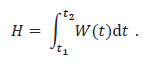
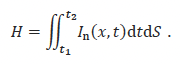
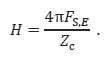
Sound energy, H, is the integral of sound power, W(t), integrated over time between t1 and t2, i.e.,
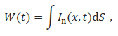
Sound power is the surface integral of the component of sound intensity, I(x, t), normal to the integration surface, S (ISO 18405: 3.1.3.14):
such that
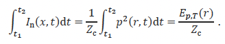
In the far field, the time-integrated squared sound pressure (equivalently, the sound exposure, Ep,T, ISO 18405: 3.1.3.5) is equal to the product of the characteristic acoustic impedance, Zc, of the medium (ISO 18405: 3.1.5.6) and the magnitude of the time-integrated sound intensity (ISO 18405: 3.1.3.10). Additionally, in spherically symmetrical space, we replace x with r where r is the distance from the acoustic centre. This provides the relationship:
Furthermore, based on far-field assumptions, one can define the energy source factor, FS,E, (ISO 80405 3.3.1.5) as
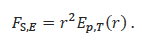
Noting that the source factor is independent of r, we can further write
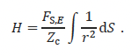
Taking the surface integral over a sphere at distance r from the acoustic centre provides a surface area of

and the result of the integral in Equation 7 as
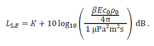
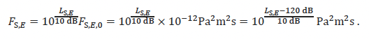
It is useful to note that the energy source factor can be written in terms of a sound exposure source level, LS,E, (ISO 18405 3.3.2.2) given by
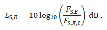
where the reference value, FS,E,0 is 1 µPa²m²s (i.e., 10-12 Pa²m²s). Consequently, it follows that
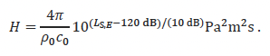
Additionally, the characteristic acoustic impedance in terms of medium density, c0, and the speed of sound, , is

Insertion of these into Equation 9 provides the quoted formula from the paper of
In this derivation, there are two crucial assumptions regarding the nature of the sound propagation. Firstly, it is presumed that there exists some region far from the source where the direct-path field amplitude varies inversely with range. Secondly, it is required that the source exists in a single medium, i.e., with a uniform characteristic acoustic impedance surrounding the source. Both need to be satisfied for the source level to exist.
With regards to these two requirements in the context of impact piling, the topic has been directly addressed in the literature. To directly quote from Ainslie et al. (2020):
"An impact-driven pile does not have a source level for two reasons. First, source level (ISO 2017) is defined in terms of the sound radiated by a source into its far field, where the propagation is spherical. For an impact-driven pile, the extent of the source throughout the entire water column from seafloor to sea surface results in cylindrical spreading from the pile wall (Dahl et al. 2012, Zampolli et al. 2013). Thus there exists no region of spherical spreading, and therefore no far field. Second, the same definition of source level invokes the concept of “a hypothetical infinite uniform lossless medium of the same density and sound speed as the real medium at the location of the source,” and therefore a source level is only defined if the source in question is in contact with a single uniform medium. The pile is in contact with a layered medium comprising water and sediment, with at least two different impedances, and therefore also does not meet this second criterion for the definition (i.e., existence) of a source level."
This distinction was noted by Zampolli et al. (2013), where it was written that “…the pile should not be represented by a point source, but rather by a conical Mach wave”. The formulation that followed provides an expression for the acoustic energy in the water column as a function of range that considers the angled wavefront of the Mach wave between the water surface and the seafloor. This derivation was validated against the numerical model results in the paper and forms the basis of the damped cylindrical spreading model (Lippert et al. 2018).
In the case of the impacted pile, as stated, there is no far field and no source level. The total sound energy of the piling pulse is dependent on the location of the surface over which sound power is integrated regardless of whether the pile is slightly embedded in the seabed or driven almost entirely in. As the apparent sound energy varies with the integrating surface, rather than the constant value achieved with the point source case, Use of Equation 13 in the context of piling leads to errors that are quantified in this report.
2.1.2. Values for the energy conversion factor
As stated earlier, one significant variable in the description of the energy source level from Equation 1 is β, i.e., the ECF. As previously stated, it is defined as

i.e., the ratio of the radiated sound energy in the water to the input hammer energy. The ECF is significant in that it represents many aspects of the piling situation and directly controls the acoustic output of the system. It is unclear exactly how the ECF is affected by the system inputs; however, attempts have been made to calculate the relative amount of hammer energy that is converted into acoustic energy based on both measurements and modelling.
There are only few reported instances of an energy conversion ratio in literature. The methods of calculation vary from considering the pile to be a point source and back-propagating from measurements, to calculating it directly from full finite-element models of the pile. As stated, and will be shown in more detail in Section 3, point source models are now known to be inappropriate for the back-propagation; they were, however, considered best available science 12 years ago and so were employed for pile modelling.
There is no direct way to measure the energy radiated from the pile. For field studies it is necessary to approximate the energy typically achieved using measurements of SEL close to the pile. From Equations 4 and 5 we can show that the total sound energy in the water column, H, is related to the sound exposure, Ēp,T(r), as

where the surface integral is taken over a cylinder spanning the water column. If we can assume radial symmetry and a depth-averaged value of sound exposure, Ēp,T(r), we can rewrite this as
where A = 2πrD (i.e., the surface area of the cylinder excluding ends) and D is the water depth. The energy conversion factor, β, is then provided by Equation 14.
In the report, “The measurement of the underwater radiated noise from marine piling including characterisation of a “soft-start” period”, Robinson et al. (2007) shows results for the driving of a 2 m diameter, 65 m long pile using hammer energies from 80 kJ to 800 kJ into chalk with local water depths ranging from 8 to 15 m. The observation of the correlation between SEL at 57 m from the pile and input hammer was made with results shown in Figure 1. Here, they calculate the gradient of the line and state that “about 0.3 % of the hammer energy is converted to sound”.
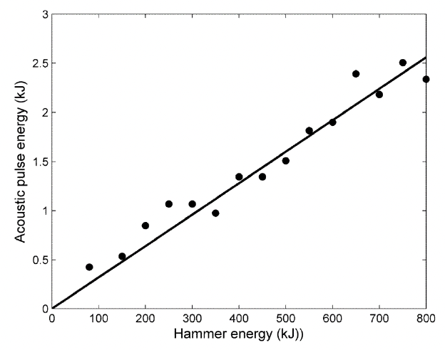
The gradient of the best-fit line has a gradient of 0.32 %.
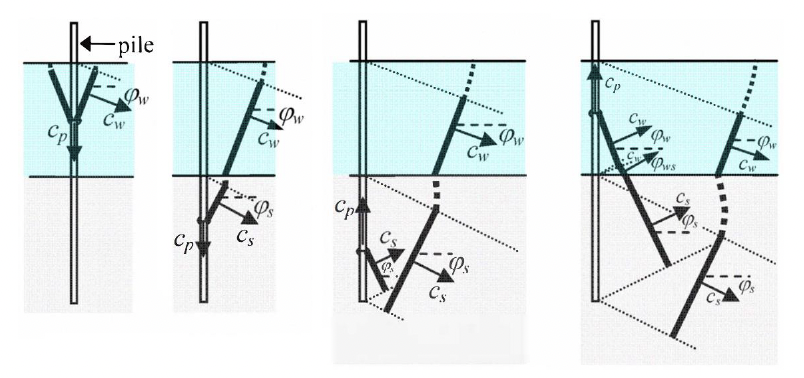
In a tour de force, Reinhall and Dahl (2011) coined the term ‘Mach’ cone, which describes the shape of the wavefront propagating from the pile; as the stress wave travels down the length of the pile, the local compressions results in a wall expansion at that point, creating an increase in pressure at the pile wall that moves down the pile at the speed of sound in the pile, thus resulting in conical wavefronts at a single angle (Figure 2). This was revolutionary as, before this, it was common to model the impacted pile as a point source; this paper showed that the point source assumption for piles was fundamentally wrong.
In their report “Beam forming of the underwater sound field from impact pile driving”, Dahl and Reinhall (2013) presented measurements made in Puget Sound of a 0.762 m diameter pile and 32 m long, driven into the sediment. Measurements were made close to the pile using a vertical line array of hydrophones. Given a hammer energy of 180 kJ, and estimated sound energy of 2400 ± 400 kJ from the complete set of line source measurements, the ECF was calculated to be between 1.11 % and 1.56 %.
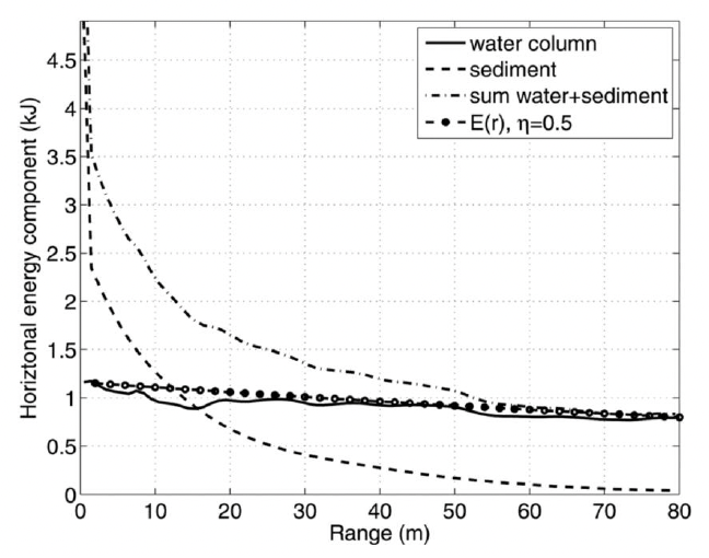
Zampolli et al. (2013) used highly detailed finite-element modelling of an impacted pile alongside an experimental set up in Kinderdijk. The pile in this case was a capped pile, 32.4 m long, with a diameter of 0.914 m, driven into medium sand. From the validated model results they calculated the energy radiated horizontally by the pile into the water to be 1.164 kJ, and the energy transferred from the hammer to the anvil to be 54.6 kJ resulting in a ratio of 2.13 %. If one considers the input hammer energy of 87 kJ rather than just that transferred to the pile, this provides an ECF of 1.33 %.
From the finite element model, Zampolli et al generated a figure of the horizontal component of the energy in the water and sediment both together and separately against a geometric spreading curve. The geometric spreading curve here is based on the description of the acoustic field in terms of the conical Mach wave rather than from a point source. The match between the finite-element model and the geometric spreading curve showed the viability of this approach.
The ratio of energy from the hammer to the sound energy is mentioned in an article by Dahl, de Jong, and Popper called “The Underwater Sound Field from Impact Pile Driving and Its Potential Effects on Marine Life” (2015). The article references the sources mentioned above to suggest that “~0.5 % of this hammer energy goes into acoustic energy that ultimately gets into the water column”. However, no additional results are presented, and so this value is presumed to be a ballpark figure given the range of calculated values from the cited references (ratios of 0.32 %, 1.11 % to 1.56 %, and 1.33 %).
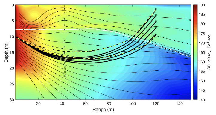
A further study into the impact pile driving sound field, with a focus on energy streamlines is one presented by Dahl and Dall'Osto (2017). The study relates to a 23.5 m long pile, with a diameter of 0.762 m, driven using an impact energy of 198 kJ. The water depth was 7.5 m, and the pile was driven to a depth of 12 m using an input hammer energy of 198 kJ. The radiated sound field was modelled using Range-dependent Acoustic Model (RAM), representing the pile as many point sources with appropriate phase delays such as to recreate the Mach cone acoustic wavefront in the water. The total energy in the water column was calculated at 60 m (water depth of 7.5 m) and 120 m (water depth of 12.5 m) from the pile using the model results. At 60 m, the total energy in the water column was 260 J, and at 120 m it was 235 J; these correspond to 0.12-0.13 % of the input energy. If one presumes a similar rate of energy loss as seen for the Kinderdijk pile in Figure 3, given the similarity in water depths, the total acoustic energy entering the water column at the pile wall is approximately 345 kJ, providing an ECF of 0.17 %.
To summarise, the results here provide values of ECF calculated from the time-integrated sound intensity integrated over a cylinder close to the pile to provide the total sound energy in the water column. Where measurements are used, the time-integrated sound intensity is estimated using results for the sound exposure level using Equation 5. The range of ECFs calculated here are between 0.17% and 1.56%; this equates to a range of 9.6 dB.
2.1.3. Use of the point-source equivalent ECF
Despite the approximations implied by treating a pile driver as a point source, forward predictions of sound fields using the point-source equivalent ECF method have appeared in reports supporting EIAs for pile driving operations. Additionally, the method has been used in other articles in a similar regard. This section provides a brief overview of its use in these works, and other points of note regarding their application. A summary of the reviewed EIAs is provided in Table 1.
| Report | Year | ECF | Notes |
|---|---|---|---|
| Beatrice Offshore Windfarm Ltd (BOWL): Piling strategy | 2015 | 1.0 % | 15log10(r) propagation |
| Seagreen Offshore Wind Farm | 2018 | 0.5 % / 1.0 % | Additional work performed using 1.0 % requested by Marine Scotland Licensing and Operations Team |
| Inch Cape Offshore Wind Farm | 2018 | 0.5 % / 1.0 % | Additional work performed using 1.0 % requested by Scottish Natural Heritage |
| Moray West Offshore Wind Farm | 2018 | 0.5 % / 1.0 % | Recalculated at 1 % as supplement to EIA |
| Moray East Offshore Wind Farm | 2019 | 0.5 % / 1.0 % | Recalculated at 1 % as supplement to EIA |
| Sizewell C Project | 2021 | 0.5 % / 1.0 % | 1.0 % only for pile diameter >2 m |
| Berwick Bank Wind Farm | 2022 | 4.0 % to 0.5 % | 4.0 % reducing to 0.5 % and others for context |
The earliest found appearance of the method was found in the Piling Strategy report for Beatrice Offshore Wind Farm (2015). The acoustic modelling was for pin piles with a diameter of 2.2 m being driven by a hammer with an input energy of 300 kJ. The summary of the acoustic modelling in the section ‘identification of impact zones’ refers to using a point-source equivalent ECF of 1.0 %, which for a 300 kJ hammer provides a per-pulse energy source level (ESL) of 205.6 dB re 1 µPa²m²s. The propagation loss was erroneously assumed to be “15log10(r)” with the only reasoning being that the operations were in shallow waters. While a 15log10(r) dependence is possible in shallow water, there is always an additional additive constant (Equation 21).
The next uses of the point-source equivalent ECF in reviewed works were for Seagreen (Farcas et al. 2018) and Inch Cape (Cefas 2018b) offshore wind farms. Seagreen featured 2 m diameter pin piles and 10 m diameter monopiles driven with hammer energies of up to 3000 kJ, while Inch Cape had 2.5 m diameter pin piles and 12 m diameter monopiles using respective hammer energies of up to 2400 kJ and 5000 kJ. The source model for each was the same as for Beatrice; the propagation, however, was modelled using an implementation of RAM, which is a well-established underwater acoustic propagation model and described more in Section 2.2.2. Propagation was calculated at 10 discrete frequencies per “1/3‑octave-band” (broadly equivalent to decidecade bands) and summed to generate the full sound field; it is not clear, however, what the maximum frequency modelled was, which would be an important aspect in the consideration of frequency-weighted sound levels. The depth-averaged sound levels were taken to generate the noise maps.
It’s notable that for these two works, the initial modelling work was carried out using an point-source equivalent ECF of 0.5 % but was revisited using a value of 1.0 % after scrutiny from the regulator (Cefas 2018c, Cefas 2018d). The effect of changing the point-source equivalent ECF from 0.5 % to 1.0 % is equivalent to doubling the hammer energy or adding 3 dB to the energy source level (and consequently to all received levels). Results in these reports are typically shown as the distances to the points where the sound level drops below a given threshold. Whilst the change of point-source equivalent ECF from 0.5 % to 1.0 % resulted in no or modest increases in some scenarios, there are extreme examples of the modelling results where PTS impact ranges for minke whales went from <50 m for the value of 0.5 % to >10 km for 1.0 % (Table 1.6, Cefas 2018d). Whilst it seems unlikely that a 3 dB increase in sound levels would result in such a change, in this example it resulted in an impact significance change from ‘Negligible’ to ‘Minor’ (Table 1.9, Cefas 2018d).
Further works from this point onwards, used 0.5 % point-source equivalent ECF as a default value. The justification for this value is based on the results highlighted in Section 2.1.2, with particular attention drawn to the comment in Dahl, de Jong and Popper (2015). Moray West had modelling for pin piles driven with a maximum energy of 3000 kJ, and monopiles with 5000 kJ (Cefas 2018a). Moray East windfarm had modelling for pin piles of a diameter of 2.5 m driven with a maximum hammer energy of 2250 kJ (Cefas 2019). Both projects used point-source equivalent ECF values of 0.5 %, and the same methods as for the previous projects. In a more recent study, for piling as part of the Sizewell C Project, a point-source equivalent ECF of 0.5 % was used for smaller diameter piles (1.0 m) whilst 1.0 % was used for the larger diameter piles (2.5 m) as a ‘precautionary’ approach (Faulkner et al. 2021). There were no details, however, as to the propagation model employed.
The increased regulatory scrutiny applied to the choice of the point-source equivalent ECF led the recent EIA for Berwick Bank (Seiche Ltd, 2022), to include further investigatory studies. The Berwick Bank report presents sound fields for numerous activities associated with the construction through to decommissioning of the wind farm. One aspect of the assessment was for impact driven piles for jacket foundations. These anchor piles had a diameter of 5.5 m with maximum (maximum hammer energy of 4000 kJ) and realistic (maximum hammer energy of 3000 kJ) scenarios defined. Additionally, these pin piles are driven such that only a small portion of the pile remains above the seabed rather than the monopile construction consider thus far.
Because of the uncertainty around an appropriate choice of point-source equivalent ECF the authors provided results considering:
- a constant conversion factor of 1 %;
- a reducing conversion factor from 10 % to 1 % (based on Thompson et al. (2020)); and
- a reducing conversion factor from 4 % to 0.5 % (based on Lippert et al. (2017)).
Final results are presented for the reducing conversion factor from 4 % to 0.5 % given the ‘best balance of realism and precaution’. It is noted, however, that Lippert et al. (2017) do not provide direct calculations of the ECF, nor reference it in the paper. What is presented by Lippert et al., however, is the measured SEL normalised to a hammer energy of 2000 kJ at 750 m from the pile as function of penetration depth. One notable outcome is the observation that for the period where the pile was entirely below the water line, the SEL reduced by 2.5 dB per 50 % reduction of the remaining pile length in the water column.
It is stated that the conversion factors have been derived following further analysis of the Lippert data; although no details are provided as to the methods applied, it is likely that the same propagation model used to generate sound fields was used to back-propagate the Lippert et al. results to generate a point source level, from which a point-source equivalent ECF can be calculated using Equations 13 and 14 yielding values between 0.5 % and 2.0 %. Further adjustments were made to the conversion factor based on the pile length exposed to the water, increasing the upper value to 3.5 %; this is based on the assumption that the energy radiated is approximately proportional to the wetted portion of the pile.
The propagation model used in the Berwick Bank EIA departs from the PE model approach. Instead, an energy flux model derived by Weston (1976) is used. Its use in this context is described further in Section 2.2.3.
As stated, the point-source equivalent ECF has been used in articles outside of environmental impact assessments. The point-source equivalent ECF method (using a value of 0.5 %) was also used for forward predictions in an article by Graham et al. (2019). In the supplementary material of the article, the propagation model described is as before with the inclusion of a separate high-frequency model based on a point-source energy-flux model for 1.25 kHz and higher. The modelling results were compared against measurements at 2.0, 7.6, and 10.2 km. For broadband sound levels, it was found that per-pulse error in the predictions were 6.6, 2.0, and 0.8 dB re 1 µPa²s respectively.
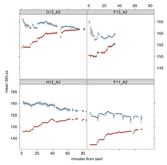
In the study “Balancing risks of injury and disturbance to marine mammals when pile driving at offshore wind farms”, Thompson et al. (2020) provide analyses of piling operations involving four 35 to 45 m long piles, each with a diameter of 2.2 m driven by a hammer with energies ranging from 266 kJ to between 744 kJ and 1735 kJ. Sound level predictions were made for four piles using the point-source equivalent ECF method for receivers between 0.8 and 3.8 km from the piling operation at 2 m above the seabed. It was found that sound levels reduced for increased penetration depths given the same hammer energy input and that low-energy-low-penetration impacts resulted in greater sound levels than high-energy-high-penetration impacts. Consequently, the point-source equivalent ECF model, which generates “source levels” using only the hammer energy and a fixed value of β, provided a poor fit to the measured results (Figure 5).
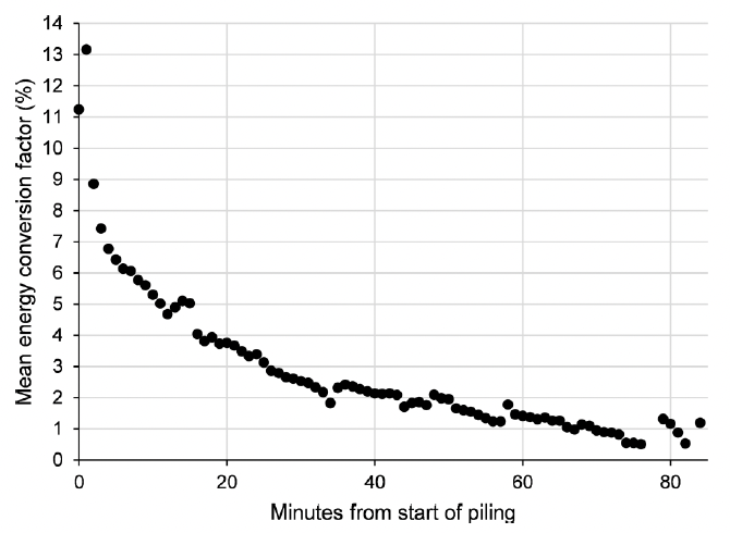
Of note, is that the paper also provides calculations of what the point-source equivalent ECF ‘should’ have been to generate the observed received levels. Although the exact process is not documented it appears that the propagation loss between the idealised point source and the receiver has been calculated to determine a source level and consequently used to determine a value for β throughout the piling sequence (Figure 6). Calculated values are between 13.2 % at the start of piling and 0.5 % towards the end. The calculated values at the start of the sequence are an order of magnitude higher than those obtained by other researchers, although the method by which the values are derived is unclear.
It is noted that there have been no formalised methods for calculating the point-source equivalent ECF. It is clear, though, that the calculation is different from those discussed in Section 2.1.2. While it is fair to say that the amount of energy converted to acoustic energy is of the order of 1 % in many cases, there appear to be a wide range of results even for a single pile operation, where many elements likely to affect the point-source equivalent ECF (i.e., hammer parameters, pile parameters, and environment) are kept constant. The implication is that, even if using Equation 1 to calculate a source level were appropriate, it is currently unknown how to accurately generate a suitable value of point-source equivalent ECF.
As shown in Table 1, the value for point-source equivalent ECF in almost all cases has been either 0.5 % or 1.0 % with 1.0 % being considered a conservative value. The sound field differences between using 0.5 % and 1.0 %, however, can be very large indeed. Additionally, as shown in the previous section, there are many examples of where the calculated point-source equivalent ECF deviates from this substantially, often by an order of magnitude. The conclusion is that using a default point-source equivalent ECF value for all piling, is unlikely to provide robust sound field results.
No mention has been made regarding usage of the point-source equivalent ECF method in terms of predicting peak sound pressure levels. The approach adopted in these works has been to use empirical linear equations that relate the peak sound pressure level to the sound exposure level by Lippert et al. (2015). The use of these correlation equations is not under scrutiny and so are not reviewed here; however, they have been shown to provide very reasonable results and no concern is raised on the use of these equations where calculations of the SEL is reliable.
2.2. Sound Propagation Models
Following a description of the sound source, it is then necessary to characterise how the sound propagates through the environment. This section provides a very brief introduction to the more common model types that are used for underwater sound propagation. Additionally, further information is provided on RAM (an implementation of the parabolic equation model type), and energy flux models, both of which have been used in the propagation of sound from piling, including those covered in the modelling in Table 1.
2.2.1. Propagation model types
The propagation of sound, when considering standard linear acoustics, is fundamentally governed by what is known in physics as the wave equation. By solving the wave equation, given certain specified boundary conditions, one can characterise the sound field at all places and at all times. The equation relates the spatial variation of an acoustic parameter, typically sound pressure, to temporal variations in that same parameter. In its standard form, the equation is difficult to solve for general cases. There are techniques, however, that make the process easier. Principally, if one assumes the sound to be at only a single frequency, the time element can be removed from the wave equation. Doing this provides a simpler function known as the Helmholtz equation that describes sound propagation at a specific frequency. The Helmholtz equation is more readily solved, and typically models would calculate the sound field for each modelled frequency separately then sum them to generate the result for all frequencies.
Acoustic models generally differ in how they solve the Helmholtz equation. These can include, but are not limited to, the following:
- Parabolic equation (PE) models,
- Ray- or beam-tracing models,
- Wavenumber integration models,
- Normal mode models,
- Energy-flux models.
A full discussion of how the models are derived is beyond the scope of this work, but detailed descriptions can be found in literature such as Jensen et al. (2011). Each model type has its strengths and weaknesses, and it should be noted that no single model is the best across all situations (Wang et al. 2014). Table 2 shows the list of model types and their applicability to different acoustic problems from Etter (2012) with additions.
The piling pulse typically has a spectrum with a peak between 100-150 Hz; consequently, a model capable of handling lower frequencies is better suited than a high-frequency model. Given the environments where one finds wind farm installations, one typically requires a model that is effective in shallow water. In the context of piling, where the principal frequency has wavelengths of between 10 and 15 m, shallow water would correspond to water depths associated with most of the continental shelf (up to approximately 200 m). Finally, it is often desirable to include bathymetric features, particularly for longer range propagation; thus, range-dependent models (i.e., ones that can handle changes in the water depth with a change in distance) are better suited. Based on Table 2, models based on the parabolic equation are most likely to yield useful results in these situations. For cases where there is little change in bathymetry, however, normal mode, wavenumber integration, and energy flux methods are very applicable.
| Model type | Application | |||||||
|---|---|---|---|---|---|---|---|---|
| Shallow water | Deep water | |||||||
| Low frequency | High frequency | Low frequency | High frequency | |||||
| RI | RD | RI | RD | RI | RD | RI | RD | |
| Ray tracing | - | - | La/s | A&p | La/s | La/s | A&p | A&p |
| Parabolic equation | La/s | A&p | La/s | La/s | La/s | A&p | La/s | La/s |
| Normal mode | A&p | La/s | A&p | La/s | A&p | La/s | La/s | - |
| Wavenumber integration | A&p | La/s | A&p | La/s | La/s | La/s | La/s | La/s |
| Energy flux | A&p | La/s | A&p | La/s | La/s | - | La/s | - |
| Hybrid normal mode energy flux | A&p | La/s | A&p | La/s | A&p | La/s | A&p | La/s |
"-" - Not Suitable
La/s - Limited in accuracy or speed of execution
A&p - Accurate and practical
2.2.2. Parabolic equation models
From Table 2, as stated, parabolic equation models are a good fit for modelling the radiated sound field from marine impact piling. The parabolic equation method presumes that the energy travelling away from the source is substantially greater than any back-scattered energy, such that one solves an outgoing wave equation rather than a more complicated elliptic boundary-value problem. Consequently, the computation is easier and typically has negligible accuracy loss due to the slowly varying environments commonly encountered in oceanic situations. Range dependency is implemented by simply representing the region as a series of range-independent regions, with a level of accuracy dictated by the resolution of these subregions.
One such implementation of the parabolic equation method is the Range-dependent Acoustic Model (Collins 1993), commonly referred to as RAM. One aspect is the initial condition, or the sound field very close to the source location, which includes a singularity at the source depth representing the point source. Unless other allowances are made, RAM calculates the sound propagation from a single point source and requires a specified depth for this point from which sound is emitted.
In the reviewed EIAs, the authors state that the model used is based on RAM but provide no source depth for the point source, or any suggestion that modifications had taken place to implement a line source. The reference for the model (Farcas et al. 2016), however, makes the assertion that “…this point source approximation can still produce reasonable predictions even for large sources such as monopiles or ships”, and refers to a source depth in the text indicating that the model used was a point source model.
2.2.3. Energy flux models
Another approach to calculating the losses associated with the propagation of sound is presented in the work by Weston (1976). By making a number of simplifications, including uniform sound speed profile, a lossless medium, smooth and slowly-varying bathymetry, and source and receivers far from the boundaries, a set of equations are defined that specify propagation loss in four regions: spherical spreading, channelling or cylindrical spreading, mode-stripping, and single-mode. As the equations do not increase the number of calculation steps with increasing frequency it is often substantially faster at higher frequencies than more complex models.
The equations describing Weston’s original model are based on the energy flux method and provide depth-independent (i.e., depth-averaged) results only. Given the requirement of a uniform sound speed, these solutions are often limited to shallow waters where water column refraction effects are negligible. Bathymetric variations are included in the form of an effective water depth, which is one that would generate the same combined reflection losses at a given range as the true bathymetry.
The approach by Weston has been extended to include consideration of the source and receiver depths and the effects of ray convergence from sea water refraction (Harrison 2013, Sertlek and Ainslie 2014). Hybrid modelling approaches such as combinations of normal mode and energy flux models can provide a similar accuracy to incoherent mode sum for the range dependent environments without requiring long computational times (Sertlek et al. 2019). While the original work of Weston presumes an omnidirectional source, the energy flux method has been extended to a source with directivity in the sagittal plane (de Jong et al. 2019). This was originally introduced in the work by Zampolli et al. (2013) which included directivity in the form of the Dirac delta function limiting propagation to a single angle, i.e., that of the conical Mach wave. This formulation of the energy flux equations, limiting sound propagation to a single angle, was further elaborated into the DCS model (Lippert et al. 2018).
Consequently, similarly to RAM, energy flux models can be used to accurately predict the sound propagation provided the assumptions in its used are valid. The original derivations in Weston (1976), and referenced to in the Berwick Bank EIA (Seiche Ltd, 2022), are based on an omnidirectional source, i.e., a point-source model. While there exist modelling developments that take the unique nature of the impacted pile source into account, they do not appear in the EIAs reviewed as part of this project.
2.3. Review Summary
This section has provided an overview of the ECF as applied to piling, and the point-source equivalent ECF used in the reviewed reports, as well as some of the background to the source prediction and propagation methods. There are concerns with two separate aspects of the adopted approaches in models using the point-source equivalent ECF.
Firstly, with regards to the sound propagation, although validated and well-established models are used, the lack of consideration for the source geometry will lead to inaccuracies in the outputs; the illustrative differences between propagation from a point and from a line is discussed extensively in Section 3.
Secondly, presuming Equation 1 to be an appropriate method, the selection of point-source equivalent ECF is somewhat arbitrary. A limited number of calculations of the ECF have yielded results from 0.17 % (Dahl and Dall'Osto 2017) to 1.56 % (Dahl and Reinhall 2013), which equates to a range of 9.6 dB. The difference between values of β of 0.5 % and 1.56 % is 4.9 dB, indicating that equivalent source levels may be underpredicted by that much based on the small set of calculated ECF values.
Using undocumented methods, point-source equivalent ECF values have been calculated to be as high as 13 % (Thompson et al. 2020). There has been little attempt to determine the factors controlling the point-source equivalent ECF, and any relative importance of the possible inputs. Additionally, even whilst restricting values of the point-source equivalent ECF to 0.5 % and 1.0 %, there are examples of very large differences in the distances to modelled isopleths corresponding to sound level thresholds.
Contact
Email: ScotMER@gov.scot
There is a problem
Thanks for your feedback