Migration routes and behaviour of Atlantic salmon and sea trout around operational wind turbine arrays in the Moray Firth, Scotland

An acoustic tracking study into the movements of Atlantic Salmon (Salmo salar) and Sea Trout (Salmo trutta) on migration through operational offshore wind farms in the Moray Firth, Scotland.


3. Results

Atlantic salmon smolts

Timing and duration of river emigration

The proportion of tagged smolts that out-migrated from the River Wick was similar in Y1 and Y2 with 88% and 90% reaching Wick harbour, equating to a freshwater loss rate of 1.1% km-1 and 0.9% in Y1 and Y2, respectively. Individuals took a median of 5 days 23h 24 minutes (range 11 h 17 minutes – 15 days 11 h 46 minutes) (Y1) and 4 days 20 h 24 minutes (range 6 h 29 minutes – 25 days 23 h 17 minutes) (Y2) after release to reach Wick harbour.

Temperature and depth (pressure) data (available for Y2 only) suggested that two salmon were preyed on by mammals within Wick harbour. Recorded temperatures rose rapidly from approximately 10°C to in excess of 30°C, concurrent with depth profiles suggesting rapid diving movements (Figure 2).
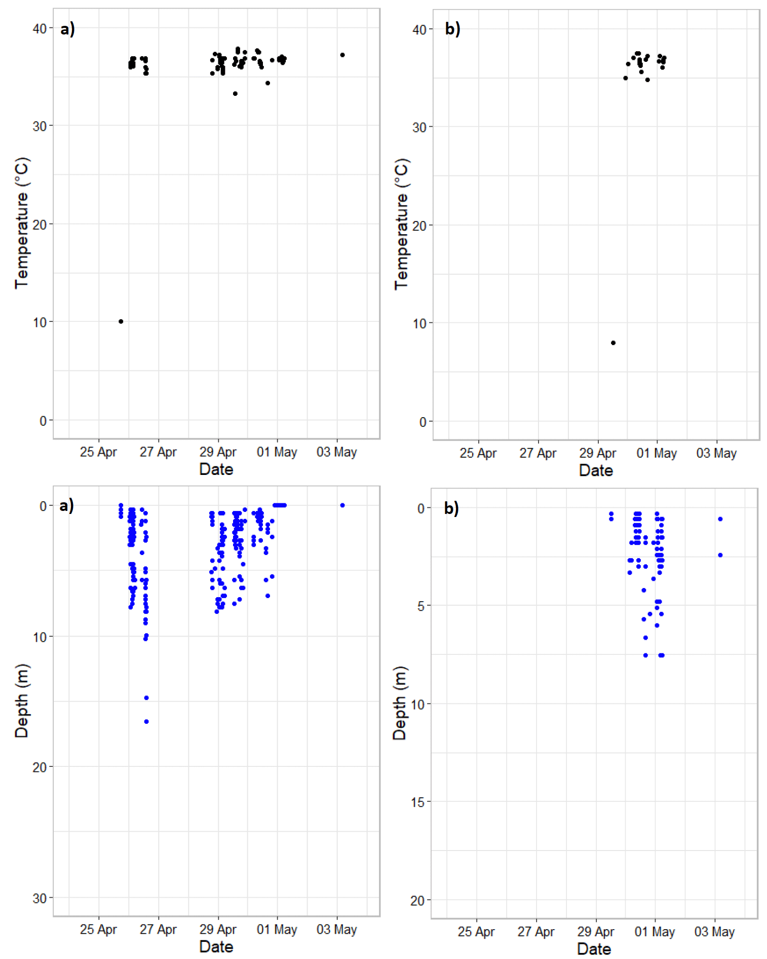
Figure 2: Temperature and depth time series graphs from two salmon post-smolts (a & b) presumed to have been preyed on by a mammalian predator within Wick Harbour in 2024.
Temperature a) Scatter plot showing temperature readings in degrees Celsius over dates from 25 April to 3 May, with most temperatures clustered between 35°C and 38°C. Two distinct clusters appear around 26 April and 30 April to 1 May, with one outlier near 10°C on 25 April. Temperature b) Scatter plot showing temperature readings in degrees Celsius over dates from 24 April to 3 May. Most data points cluster around 35-38°C between 29 and 2 May, with one notable outlier near 8°C on 29 April. Depth a) Scatter plot showing depth measurements in metres over dates from 25 April to 3 May, with depth values mostly clustered near 0 to 10 metres. Blue dots represent individual data points, indicating fluctuations in depth primarily between 0 and 10 metres, with few outliers reaching deeper levels. Depth b) Scatter plot showing depth measurements in metres over time from 25 April to 3 May, with data points clustered mostly between 0 and 7 metres depth around 1 May. Blue dots represent individual depth readings, highlighting a concentration of measurements near surface level.

A total of 94 post-smolts in Y1 (87%) and 80 post-smolts in Y2 (80%) were assumed to have successfully entered the Moray Firth, having either been detected on the outer line of receivers in Wick Bay (173 individuals) or detected in the marine array after passing through the outer line without detection (1 individual). Most post-smolts passed through Wick Bay without delay, with 95% residing for 24 h or less (Figure 3). Outmigration occurred almost exclusively during darkness with movements predominantly associated with the period from 2100 to 0100 (Figure 4). In Y1, 39 individuals exited on an ebb tide and 55 on a flood tide compared to 37 exiting on an ebb and 42 exiting on a flood tide in Y2 (excluding the one individual for which we do not know the precise time of departure).
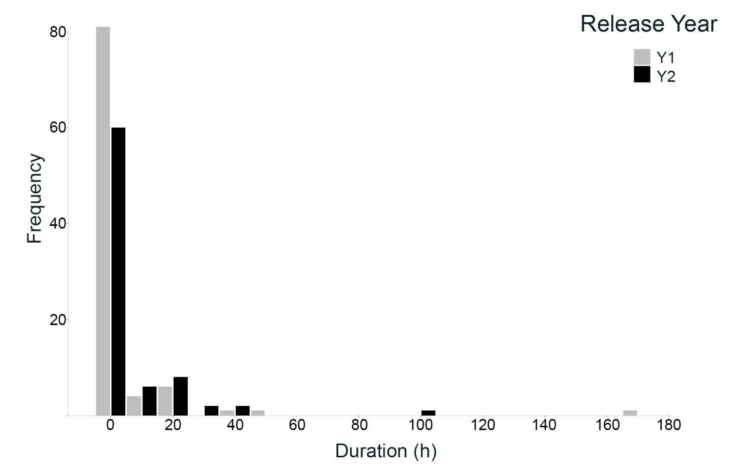
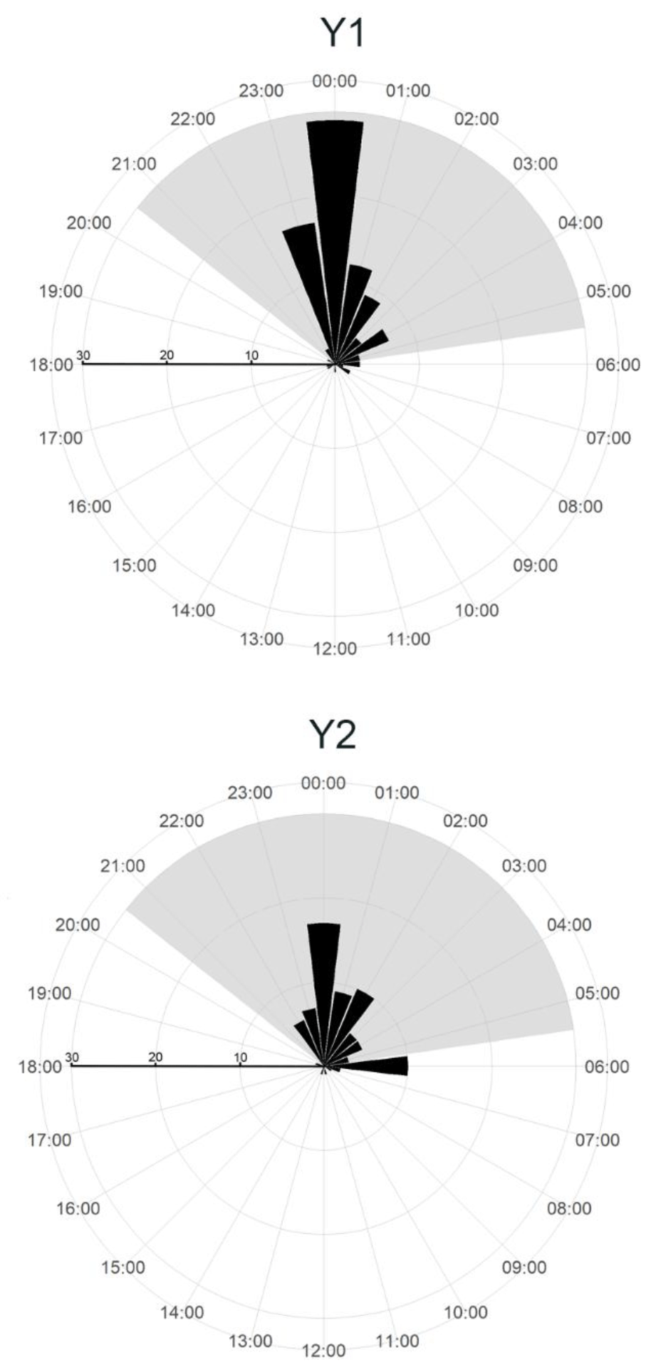
Figure 3: Duration (h) salmon post-smolts spent within Wick harbour and bay before assumed successful emigration to the Moray Firth (denoted by last detection on outer receiver line in Wick Bay) (n = 173)
Bar chart comparing frequency of durations in hours for two release years, Y1 and Y2. Most durations are under 10 hours, with Y1 peaking around 80 and Y2 around 60, while longer durations show minimal frequency for both years.
Figure 4: Rose diagrams depicting the time of day at which salmon post-smolts departed Wick Bay and entered the Moray Firth in Y1 (n = 94) and Y2 (n = 79). Grey shading indicates the period between sunset and sunrise.
Two polar bar charts display data distributions over 24 hours for Y1 and Y2. Both charts use black bars on a grey radial grid with hour labels around the perimeter, showing peak values around midnight for Y1 and early morning for Y2.

Marine migration characteristics

A total of 37 emigrating salmon post-smolts in Y1 (39%) and 39 in Y2 (49%) were subsequently detected by the marine receiver array. In both years, most of the first offshore detections were on the North Line of receivers: 51 % in Y1 and 49 % in Y2 compared to 24 % and 10% on the South Line in Y1 and Y2, respectively (Figure 5). The time between emigration into the Moray Firth and first detection in the marine array ranged from 7 h 56 minutes to 5 days 1 h 55 minutes (median 26 h 28 minutes). Neither current speed or bearing at Wick Bay entrance, nor release year, had a significant effect on the location of first detection after leaving Wick Bay.
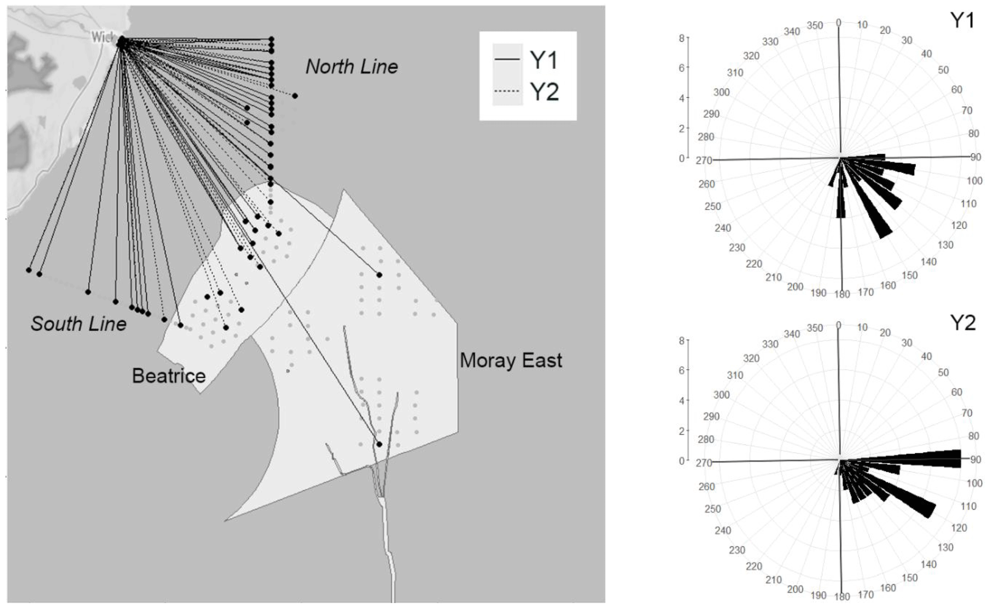
Figure 5: Map (left) and rose diagrams (inset) depicting assumed straight line swim bearings of salmon smolts that departed Wick Bay and were subsequently detected by receivers in the marine array in the Moray Firth in Y1 (n = 37) and Y2 (n = 39)
Map and two polar bar charts showing spatial distribution and directional data for Y1 and Y2. Map highlights North Line, South Line, Beatrice, and Moray East areas with solid and dotted lines representing Y1 and Y2, while charts display frequency peaks around 90° for Y1 and near 180° for Y2.

The time between the first and last detections in the marine receiver array ranged from 1 s to 7 days 14 h 53 minutes (median 1 h 7 minutes) in Y1 and from 5 minutes 17 s to 6 days 17 h (median 7 h 48 minutes) in Y2. In both years, receivers in the north line detected the highest number of individuals (Figure 6).
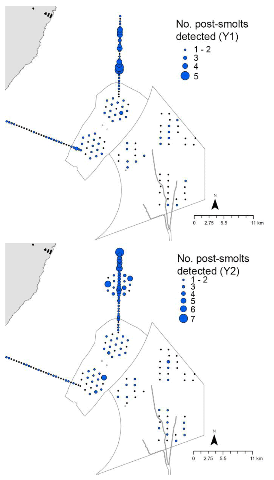
Figure 6: Number of salmon post-smolts detected per receiver within the whole marine array, including the turbine zones of the Beatrice and Moray East offshore wind development sites in Y1 and Y2
Two side-by-side maps display distribution of post-smolts detected in years one and two, using blue circles of varying sizes to represent quantities from one to seven. Both maps include a scale bar, north arrow, and labelled legend, highlighting increased detections in year two compared to year one. Two maps display spatial distribution of post-smolts detected in years one and two, using blue circles of varying sizes to represent numbers ranging from 1 to 5 in year one and 1 to 7 in year two. Both maps include a legend, north arrow, and scale bar.

Association with offshore wind development sites

Just under half of the post-smolts detected within the marine array were detected within the OWDs; a total of 17 post-smolts in Y1 (46%) and 16 in Y2 (41%), which in both years represented 16% of all smolts tagged. Sixty one percent of those 33 post-smolts were not intercepted by the North Line or South Line, i.e. their first marine detection was within a OWD boundary, mostly within Beatrice. By contrast, most of their last detections were in Moray East (Figure 7).
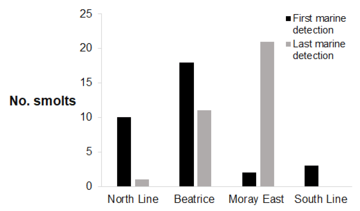
Figure 7: Region of first and last detections within the marine array for the 33 post-smolts which entered the Beatrice and Moray East OWDs (Y1 & Y2 combined)
Bar chart comparing number of smolts detected at first and last marine detection across four locations: North Line, Beatrice, Moray East, and South Line. Black bars represent first detections, with Beatrice highest at 18 smolts, while grey bars represent last detections, with Moray East highest at 20 smolts.

Post-smolts resided within the OWDs for a minimum total duration of between 1 s and 4 h 44 minutes (median 35 minutes 31 s), with no significant difference between years (W = 128, p = 0.79, n = 33). The spatial pattern of residency in the turbine areas indicated longest durations within the Beatrice OWD (Figure 8). Individual residence events lasted from less than 1 s to 2 h 22 minutes, with a median duration of 3 minutes 30 s.
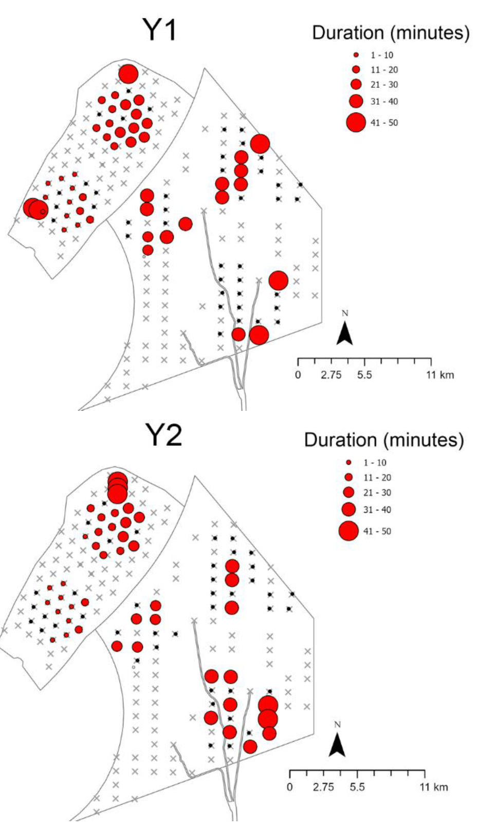
Figure 8: Total duration of residence events of salmon post-smolts within the turbine zones of the Beatrice and Moray East offshore wind developments during Y1 (n = 17) and Y2 (n = 16)
Two side-by-side maps display duration of events in minutes using red circles of varying sizes, with larger circles indicating longer durations ranging from 1 to 50 minutes. Both maps, labelled Y1 and Y2, feature a legend for circle sizes, a north arrow, and a scale bar showing distances up to 11 km, highlighting spatial distribution and duration differences across the mapped areas.

Residency durations determined by summing the duration of individual residence events denotes certain but minimum time spent by fish in the OWDs because there was not complete receiver coverage of the turbine arrays, hence fish may have been in the vicinity of the turbines but undetected. The temporal pattern of detections suggests most post-smolts were present within the OWDs for one or two discrete events (Figure 9, Figure 10 ). The temporal spread of detections was generally longer in Y1 than Y2, spanning a period of 17 days in Y1 and 7 days in Y2.
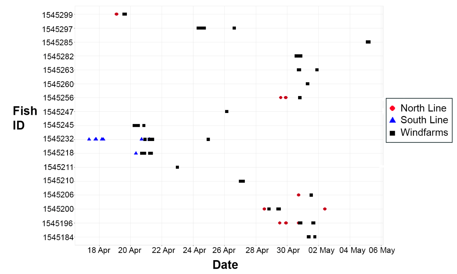
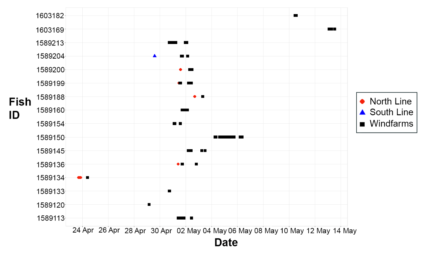
Figure 9: Temporal pattern of detections on the North Line and South Line of receivers and within the Beatrice and Moray East OWDs for post-smolts in Y1 (n = 17) that entered the OWDs during their marine migration.
Scatter plot showing fish ID tracking data over time from 18 April to 6 May, categorised by three groups: North Line (red circles), South Line (blue triangles), and Windfarms (black squares). Data points indicate individual fish detections with Windfarms group appearing most frequently and spread across the entire date range, while North and South Lines show fewer detections clustered around late April and early May.
Figure 10: Temporal pattern of detections on the North Line and South Line of receivers and within the Beatrice and Moray East OWDs for post-smolts in Y2 (n = 16) that entered the OWDs during their marine migration. Note the condensed date values on the x-axis (grey section).
Scatter plot showing fish tracking data over time from 24 April to 14 May, with Fish ID on vertical axis and Date on horizontal axis. Data points include red circles for North Line, blue triangles for South Line, and black squares for Windfarms, highlighting fish presence and movement patterns across different locations.

Movement patterns within the OWDs, including the direction and total distance travelled, were inferred using assumed straight-line paths for post-smolts detected at two or more receivers within discrete periods that were temporally separated by less than 24 h (14 fish in Y1 and 12 fish in Y2). The bearings of assumed straight line trajectories between successive detection locations (i.e. steps) showed, in both years, a clear tendency for south and south-easterly movements (Figure 11). In Y1 there was also a notable trend towards easterly and northerly swim paths; 23% of steps were on a northerly or north-easterly bearing.
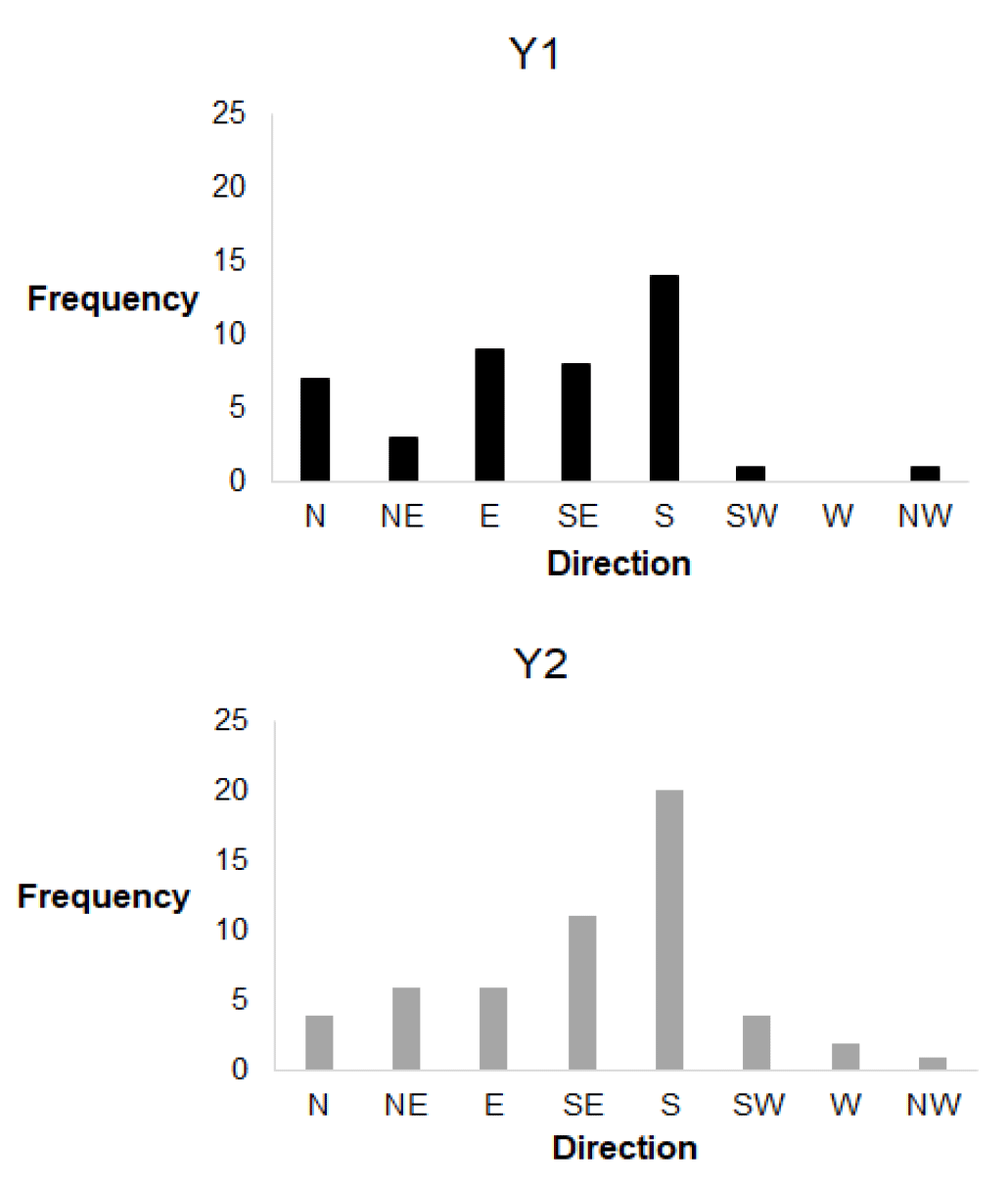
Figure 11: Frequency histograms of compass bearings of swim path steps between consecutive residence events at different receivers in the Beatrice and Moray East OWDs for 14 post-smolts in Y1 (33 steps) and 12 post-smolts in Y2 (57 steps)
Bar chart showing frequency distribution of directions labelled N, NE, E, SE, S, SW, W, NW on horizontal axis and frequency values on vertical axis. Highest frequency occurs at S with 20, followed by SE with 11, while NW has the lowest frequency of 1.

The total distance travelled by individual post-smolts within the OWDs ranged from 0.51 to 13.91 km (median 6.82 km) in Y1 and from 1.14 to 45.29 km (median 9.33 km) in Y2 (Figure 12). Individual trajectories were highly variable (Appendix 1).
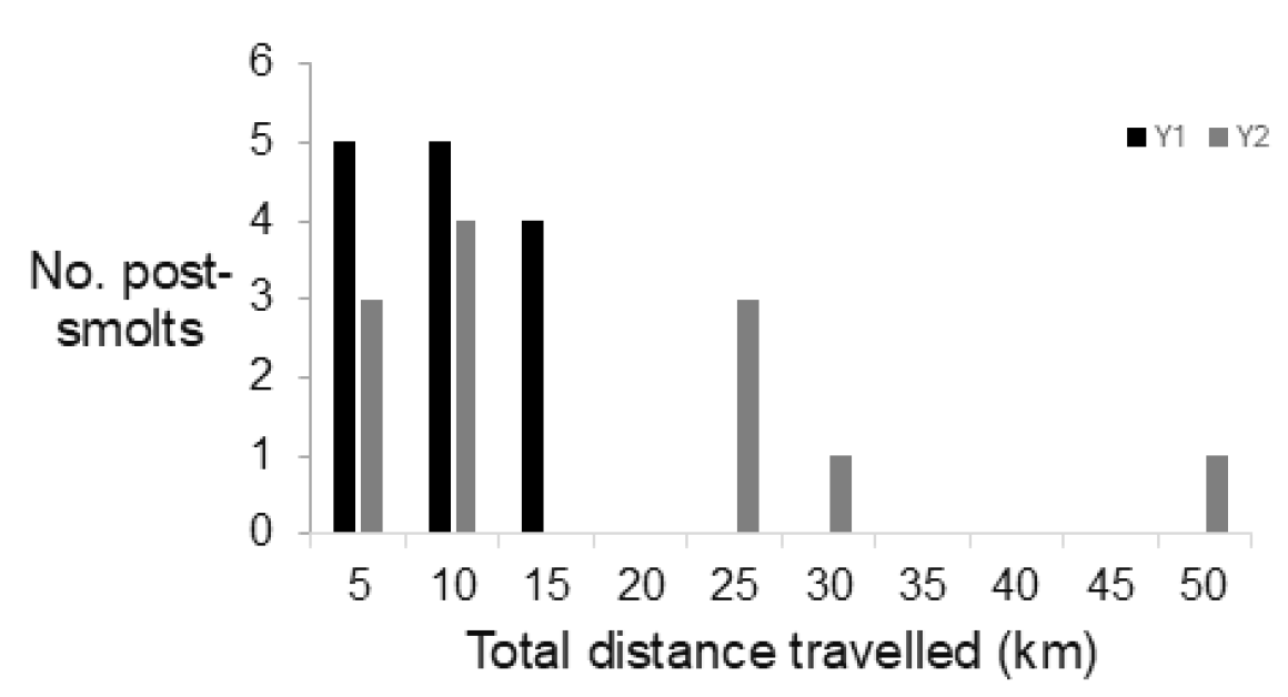
Figure 12: Frequency histogram showing minimum total distance travelled by post-smolts within the Beatrice and Moray East OWDs for 14 post-smolts in Y1 (black bars) and 12 post-smolts in Y2 (grey bars)
Bar chart comparing number of post-smolts against total distance travelled in kilometres for two groups labelled Y1 and Y2. Chart shows higher post-smolts counts for shorter distances, with Y1 consistently having more post-smolts than Y2 across all distance categories.

Temperature and swimming depth

Of the 30 smolts tagged with transmitters with temperature and pressure sensors (Y2 only), temperature data were recorded from 14 individuals (298 detections) and depth data from 15 individuals (1211 detections) while within the marine receiver array. Recorded temperatures ranged from 7.85 to 10.67°C (mean 8.52 ± 0.43 S.D.) and recorded depths were consistently within the surface layer (range 0–3.31 m) with 98% of values 2.05 m or shallower. The median swimming depth recorded during the day (sunrise to sunset) was 0.30 m (range from 0.0001 to 3.31 m) (681 values from 15 individuals). The median swimming depth recorded during the night (sunset to sunrise) was 0.0001 m (range from 0.0001 to 0.31 m). These data provide no evidence of predation on post-smolts by mammalian predators while within the marine array. Predation by ectothermic predators such as piscivorous fish cannot be ruled out, but depth profiles did not show any sudden rapid changes in depth or use of deeper waters which can be indicative of such predation.

Adult sea trout

Detections from all of the 17 adult sea trout released in Y1, and from 45 of the 52 sea trout released in Y2 were retained within analyses. The overall time difference between the first and last marine detections of individuals ranged from 25 minutes to 17 days 6 h (median 31 h 19 minutes 48 s) in Y1 and from 37 minutes 10 s to 129 days 1 h 12 s (median 2 days 21 h 22 minutes) in Y2. Fish dispersed from their release points and were frequently detected within other parts of the array; 18% and 20% of the last marine detections were in the Moray East OWD in Y1 and Y2, respectively (Figure 13 and Figure 14).
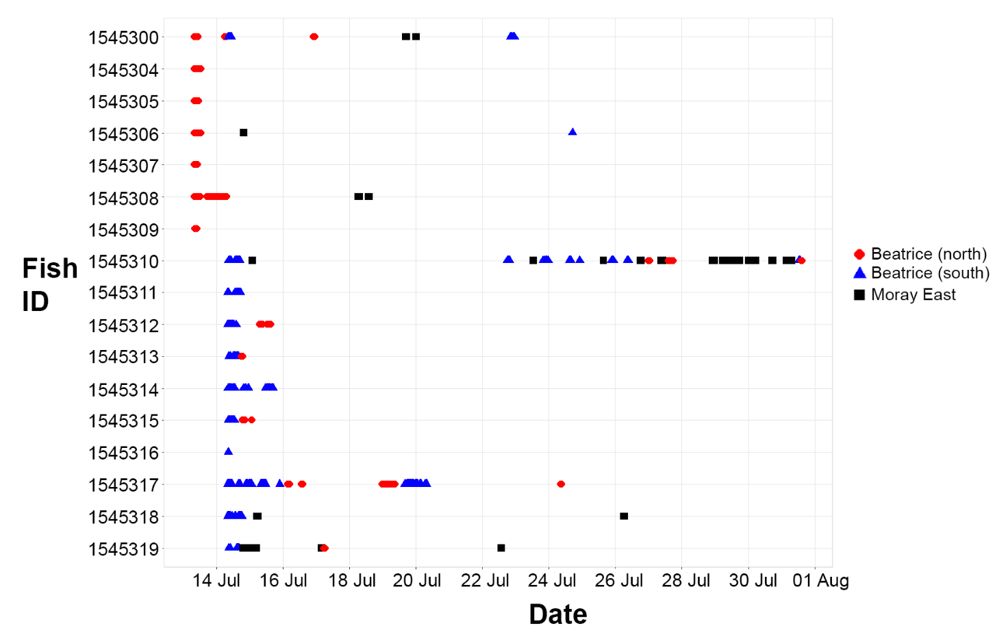
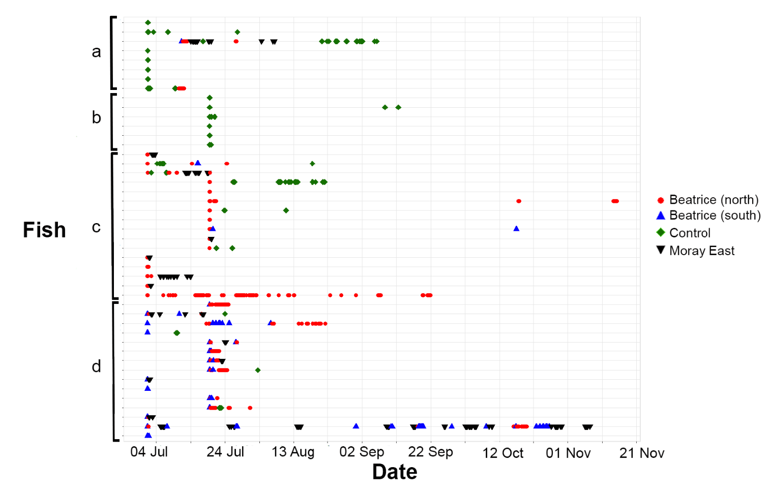
Figure 13: Temporal pattern of marine detections of adult sea trout released in Y1 (n = 17)
Scatter plot showing fish detection events over time for individual Fish IDs from 14 July to 1 August. Data points are colour-coded by location: red circles for Beatrice (north), blue triangles for Beatrice (south), and black squares for Moray East.
Figure 14: Temporal pattern of marine detections of adult sea trout released in Y2 (n = 45). Each horizontal line denotes an individual fish. Letters indicate the release location: a – “South of Control Area”; b – “Control Area”; c – Beatrice (North); d – Beatrice (South).
Scatter plot showing fish observations over time from early July to late November, categorised by four groups labeled a to d on the vertical axis. Data points use different coloured and shaped markers representing Beatrice (north) in red circles, Beatrice (south) in blue triangles, Control in green diamonds, and Moray East in black inverted triangles

Residency within the offshore wind developments

The total duration of residency events per fish within the OWDs ranged from 25 minutes 8 s to 16 h 36 minutes 36 s (median 3 h 6 minutes) in Y1 and from 10 minutes 41 s to 5 days 14 minutes 24 s (median 5 h) in Y2. The minimum total distance covered during these residencies (track length) ranged from 3.50 km to 201.32 km (median 27.47 km) and from 1.20 km to 384.60 km (median 21.76 km) in Y1 and Y2, respectively.

The longest total durations (all fish combined) were associated with receivers near the release sites in the Beatrice OWD, although there were total durations up to 2h (Y1) and 18 h (Y2) spread throughout the Moray East OWD (Figure 15). The maximum total duration per receiver was 7 h 13 minutes 12 s in Y1 and 49 h 13 minutes 48 s in Y2.
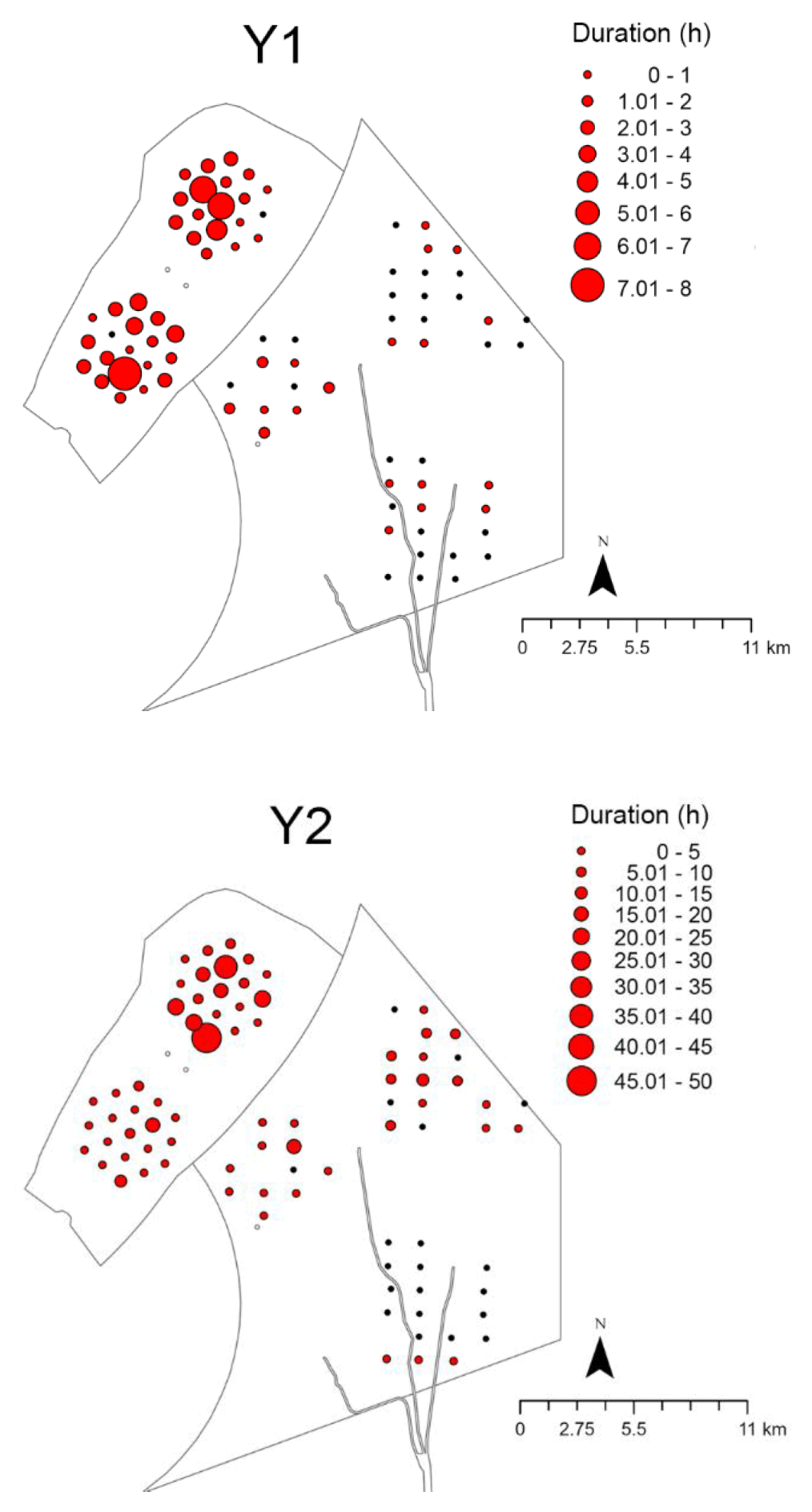
Figure 15: Total duration of residence events of adult sea trout within the turbine zones of the Beatrice and Moray East offshore wind developments during Y1 and Y2
Two side-by-side maps display spatial distribution of duration in hours, represented by red circles of varying sizes, across regions labelled Y1 and Y2. Each map includes a legend indicating duration ranges from 0-1 to 45-50 hours, with larger circles showing longer durations concentrated in northern areas.

Comparing residency and behaviour in Beatrice OWD and control area

A minimum of 12 sea trout individuals were detected, beyond the 30 minute acclimation cut-off, in each of the three comparable ‘test areas’ (i.e. identical hexagons of receivers in Beatrice North, Beatrice South and “Control Area”, see Figure 2) per year (Table 3).

Table 3: Number of adult sea trout detected in the three test areas (receiver hexagons) per year, irrespective of release location, along with minimum and maximum number of detections and average total residence duration per fish.
Year Test area No. ST detected Minimum no. detections/fish Maximum no. detections/fish
Y1 Beatrice North 13 21 826
Y1 Beatrice South 12 10 786
Y1 Control Area NA - -
Y2 Beatrice North 29 6 1920
Y2 Beatrice South 18 4 2197
Y2 Control Area 23 3 782

Residence duration in each area per fish per day ranged from less than one second to 8 h 10 minutes 48 s in Y1 and from less than one second to 14 h 40 minutes 48 s in Y2, with no difference between areas (test area explained 0.36% of residual deviance in GLMMs).

A Roaming Index, the average number of stations within an area visited by a fish per hour, used to infer exploratory behaviour, did not vary between test areas for either year. Sea trout in Y2 visited a median of 2.24 and 2.40 stations h-1 in Beatrice North and Beatrice South, respectively, compared to a median of 2.90 stations h-1 in the control area. Test area was not a significant predictor of Roaming Index, explaining just 0.2% of residual deviance in GLMMs.

Depth use

Swimming depth data which were available for all 17 of the sea trout released in Y1 and 34 of the sea trout released in Y2 showed greatest use of the top 10% and bottom 20% of the water column with fish tending not to dwell in the central zones (Figure 16,Figure 17). In Y2, sea trout were most frequently detected at in water depths of 40-55 m (Figure 17).
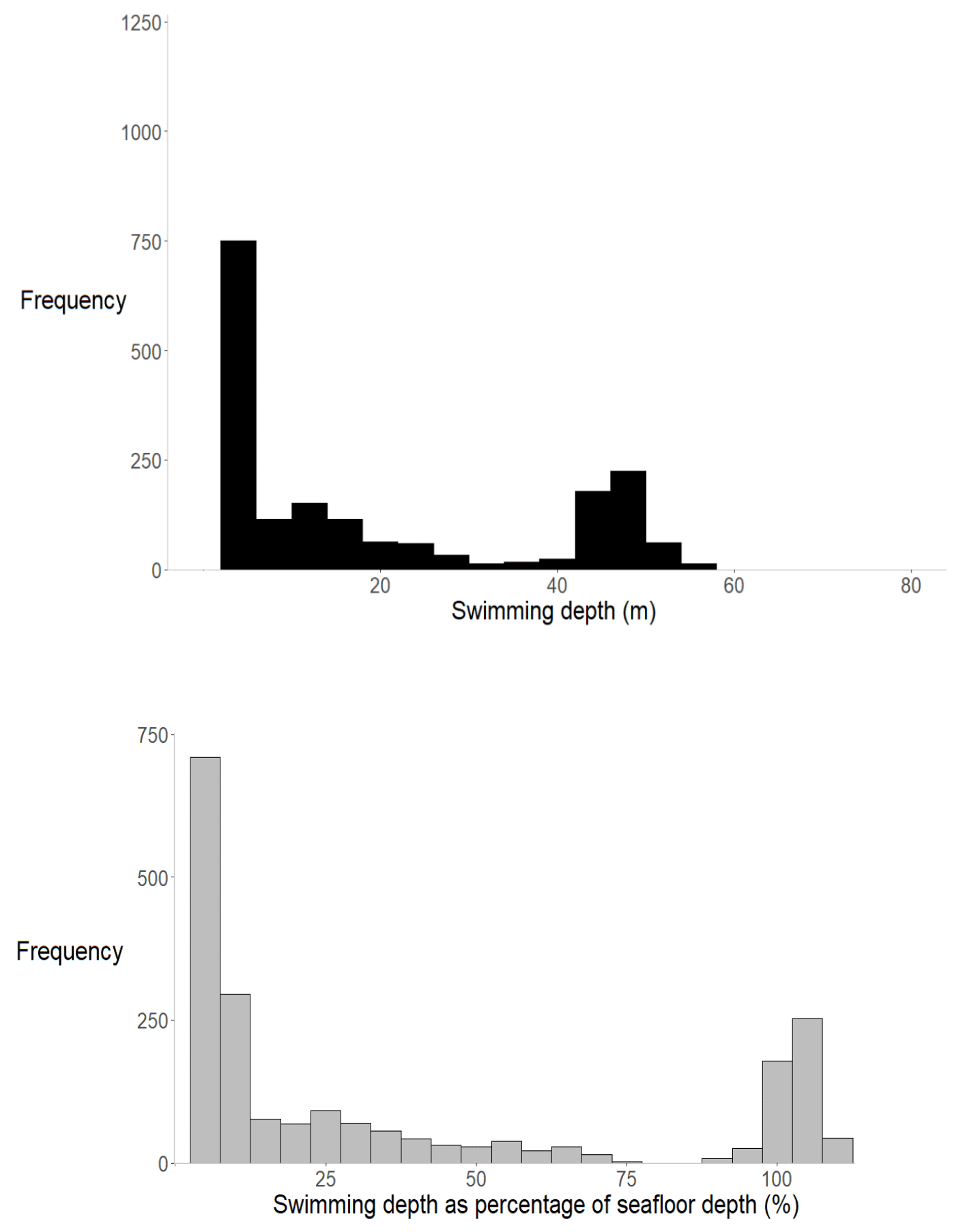
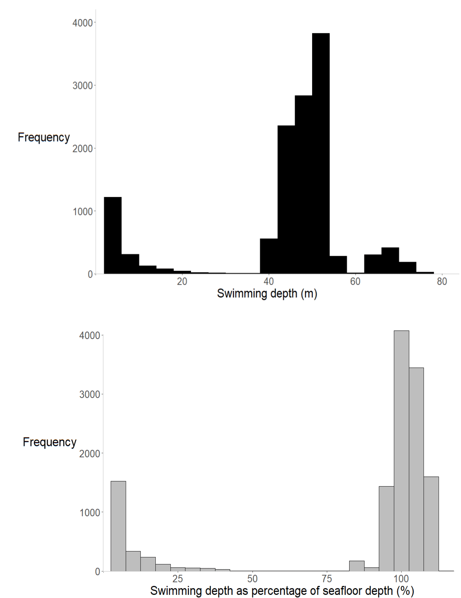
Figure 16: Frequency histograms of swimming depths expressed in m (a) and % of total seafloor depth (b) recorded from 17 adult sea trout released into Beatrice offshore wind development in Y1. Note: some % values exceed 100 due to limitations in the resolution of bathymetric data
Bar chart showing frequency distribution of swimming depths in metres, with depth on horizontal axis and frequency on vertical axis. Highest frequency occurs at shallow depths around 5 metres, with a secondary peak near 50 metres, and lower frequencies at intermediate and greater depths.
Figure 17: Frequency histograms of swimming depths expressed in m (a) and % of total seafloor depth (b) recorded from 34 adult sea trout released into the Control Area and Beatrice offshore wind development in Y2. Note: some % values exceed 100 due to limitations in the resolution of bathymetric data
Upper Bar chart showing frequency distribution of swimming depths in metres. Highest frequencies occur between 40-60 metres, with smaller peaks around 0-10 metres and 65-75 metres. Lower Bar chart showing frequency distribution of swimming depth as percentage of seafloor depth, with most data clustered near 0% and 100%. The chart uses grey bars and highlights two significant peaks, one around 0-5% and another around 95-100%, indicating common swimming depths close to surface and seafloor.

Comparison of swimming depth values recorded in both the OWDs (Beatrice and Moray East) with those from the Control Area revealed a similar bimodal distribution (Figure 18). In the OWDs, 75% of recorded depths were at 75% of seafloor depth or deeper compared to 54% of values in the Control Area, suggesting slightly less use of the deepest water depths in the Control Area.
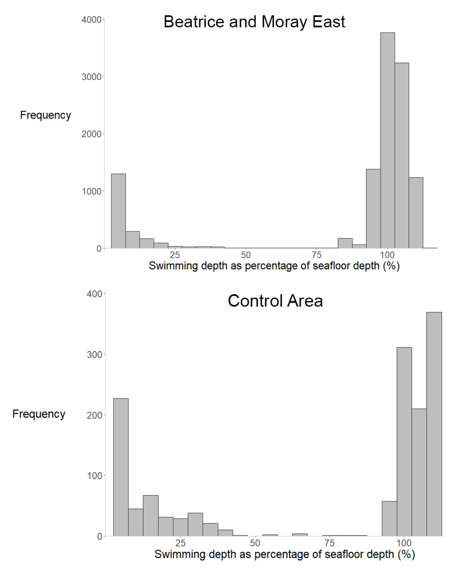
Figure 18: Frequency histograms of swimming depths expressed as % of total seafloor depth recorded from 24 sea trout detected in the Beatrice and Moray East offshore wind developments, and 15 sea trout detected in the Control Area. Note: some % values exceed 100 due to limitations in the resolution of bathymetric data
Upper Bar chart showing frequency distribution of swimming depth as a percentage of seafloor depth for Beatrice and Moray East. The chart features two prominent peaks around 0-10% and 90-110%, indicating most swimming occurs near surface or close to seafloor, with frequency values labelled on vertical axis and percentage on horizontal axis. Lower Bar chart showing frequency distribution of swimming depth as percentage of seafloor depth in control area, with x-axis ranging from 0% to 100% and y-axis showing frequency up to 400. Two prominent peaks appear near 0% and 100%, indicating most swimming occurs close to seafloor surface or at seafloor level, with fewer instances at intermediate depths.

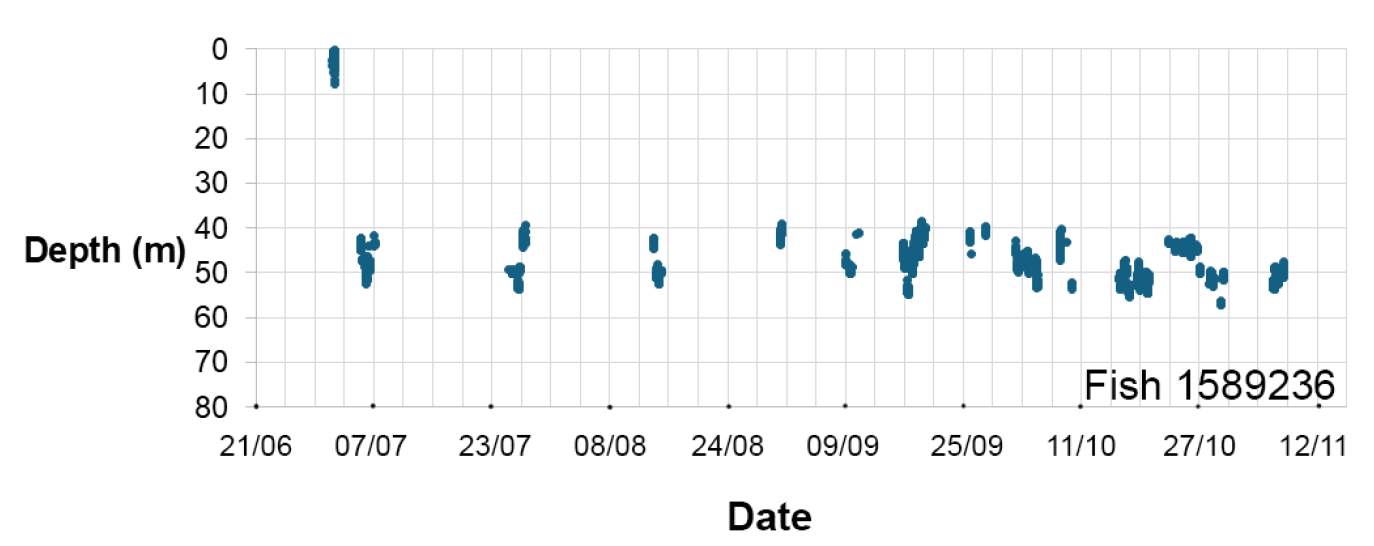
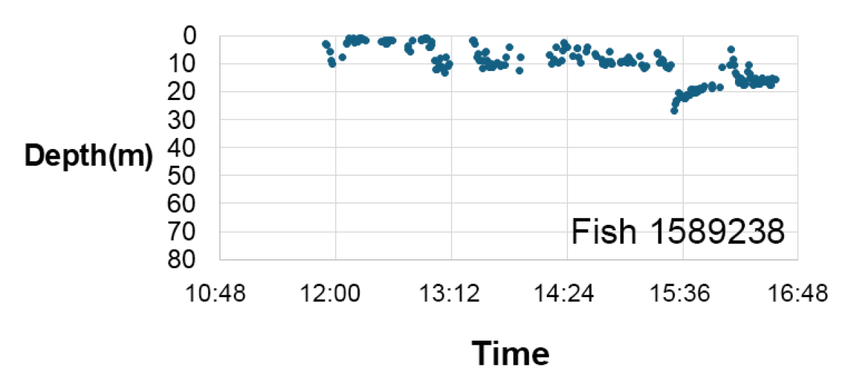
Due to depth data being collected only at the timestamps when fish were in the detection zone of a receiver, robust reconstruction of individual depth profiles was limited by temporal gaps in the detection record. However, data from a small number of fish with extended periods of near continuous detections provided more detailed insight into the range of behaviours exhibited by sea trout in the current study. These included, for example, repeated dives from the surface to depths of 25 to 30 m, which occurred exclusively during the daytime, with the fish dwelling near the surface overnight (Figure 19). Among several other fish, there was a pattern of fish spending time near the surface (hours or days) before diving to great depth (> 40 m) and remaining there for extended periods i.e. multiple days (Figure 20, Figure 21). Some fish were only detected in surface waters, with the majority of their recorded swim depths within the top 10 m of the water column (Figure 22).
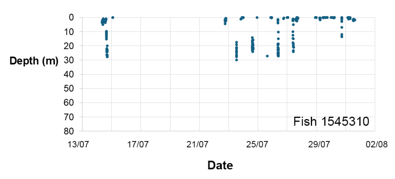
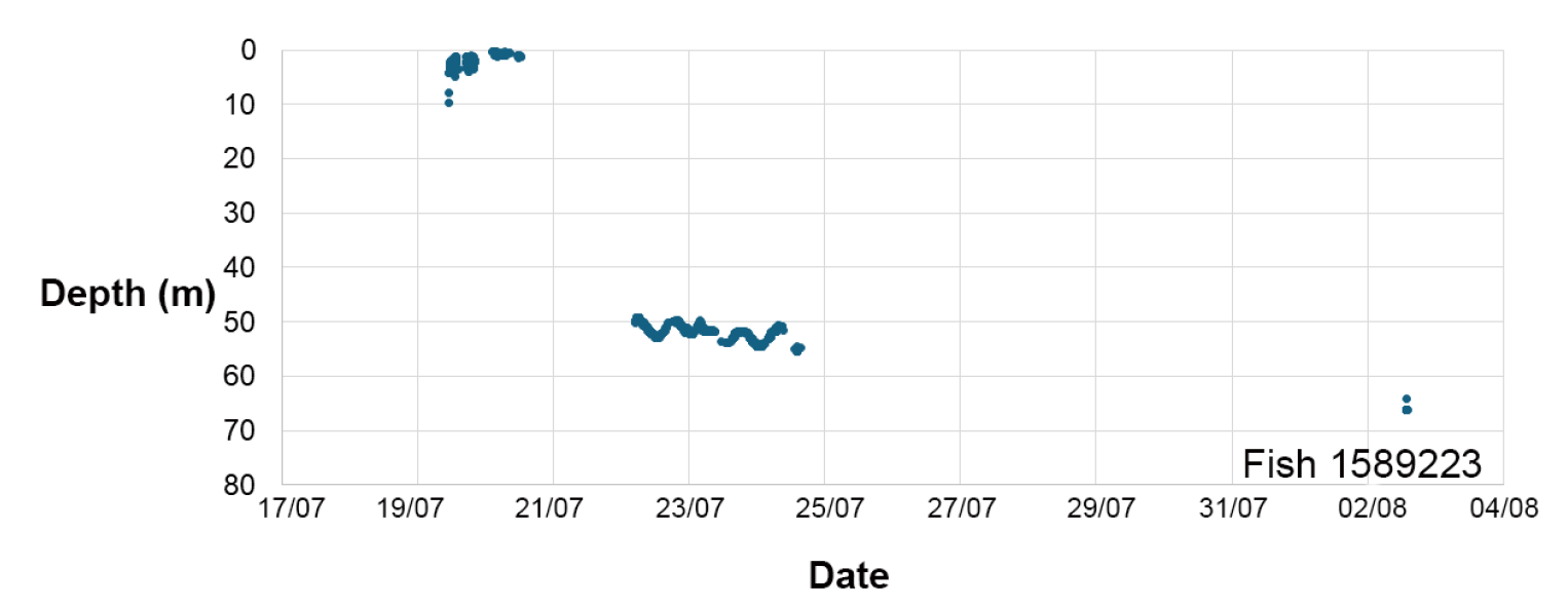
Figure 19: Swimming depth profile of an adult sea trout (Fish 1545310) detected within the marine acoustic receiver array during a period of 18 days in Y1
Scatter plot showing depth measurements of a fish tagged 1545310 over time from 13 July to 2 August. Data points cluster near surface depths between 0 and 20 metres, with intermittent deeper dives around 30 to 40 metres, indicating variable depth usage during this period.
Figure 20: Swimming depth profile of an adult sea trout (Fish 1589223) detected within the marine acoustic receiver array during a period of 15 days in Y2
Scatter plot showing depth measurements of a fish tagged as 1589223 over time from 17 July to 4 August. Data points cluster near surface depths around 0-10 meters in mid-July, shift to depths of 50-60 meters between 22 and 25 July, with a single deeper reading near 70 meters on 2 August.
Figure 21: Swimming depth profile of an adult sea trout (Fish 1589236) detected within the marine acoustic receiver array during a period of 4 months and 7 days in Y2
Scatter plot showing depth measurements of Fish 1589236 over time from late June to mid-November, with depth values mostly ranging between 40 and 60 metres. Data points are clustered with some gaps, indicating periods of more frequent depth recordings and occasional deeper measurements near surface level.
Figure 22: Swimming depth profile of an adult sea trout (Fish 1589238) detected within the marine acoustic receiver array during a period of 4 h on 1st July in Y2
Scatter plot showing depth in metres of Fish 1589238 over time from 10:48 to 16:48, with depth values mostly between 0 and 20 metres. Data points cluster near surface with a brief increase in depth around 15:36, indicating changes in fish vertical movement throughout the day.

Temperature data

Temperature data recorded by the marine receiver array fell within a narrow range in both Y1 (11.30 – 15.38°C) and Y2 (10.67 – 13.96°C) (Figure 23) and therefore provided no evidence of predation of sea trout by mammals in either year.
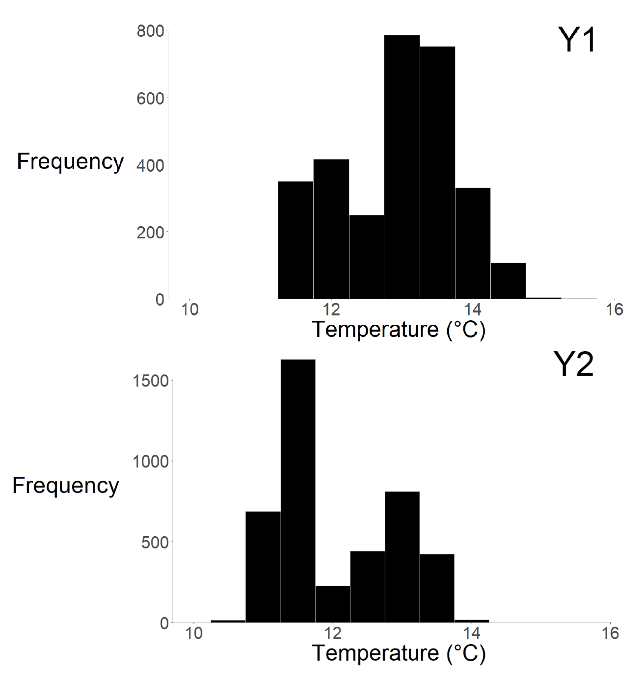
Figure 23: Frequency histograms of temperature data recorded from sea trout detected within the marine receiver array during Y1 (n = 17) and Y2 (n = 34)
Upper Bar chart showing frequency distribution of temperature readings in degrees Celsius, ranging from 10 to 16°C. Highest frequency occurs at 12°C with over 1500 counts, while frequencies at other temperatures vary between 0 and 900, indicating a peak around 12°C. Lower Bar chart showing frequency distribution of temperature readings in degrees Celsius, ranging from 10 to 16°C. Highest frequency occurs at 12°C with over 1500 counts, while frequencies at other temperatures vary between 0 and 900, indicating a peak around 12°C.

Contact

Email: ScotMER@gov.scot

Back to top